Learning Outcomes
- Use Newton’s Law of Cooling.
- Use a logistic growth model.
- Choose an appropriate model for data.
tip for success
The applications in this section rely upon all the knowledge we’ve built up from our first study of the language and notation of functions to the most recent work you’ve done in exponential and logarithmic functions.
If you need a refresher, return to Algebra Basics, the module on function basics,or any section you’ve covered with regard to modeling using functions.
Using Newton’s Law of Cooling
Exponential decay can also be applied to temperature. When a hot object is left in surrounding air that is at a lower temperature, the object’s temperature will decrease exponentially, leveling off as it approaches the surrounding air temperature. On a graph of the temperature function, the leveling off will correspond to a horizontal asymptote at the temperature of the surrounding air. Unless the room temperature is zero, this will correspond to a vertical shift of the generic exponential decay function. This translation leads to Newton’s Law of Cooling, the scientific formula for temperature as a function of time as an object’s temperature is equalized with the ambient temperature.
The formula is derived as follows:
[latex]\begin{array}{l}T\left(t\right)=A{b}^{ct}+{T}_{s}\hfill & \hfill \\ T\left(t\right)=A{e}^{\mathrm{ln}\left({b}^{ct}\right)}+{T}_{s}\hfill & \text{Properties of logarithms}.\hfill \\ T\left(t\right)=A{e}^{ct\mathrm{ln}b}+{T}_{s}\hfill & \text{Properties of logarithms}.\hfill \\ T\left(t\right)=A{e}^{kt}+{T}_{s}\hfill & \text{Rename the constant }c \mathrm{ln} b,\text{ calling it }k.\hfill \end{array}[/latex]
A General Note: Newton’s Law of Cooling
The temperature of an object, T, in surrounding air with temperature [latex]{T}_{s}[/latex] will behave according to the formula
[latex]T\left(t\right)=A{e}^{kt}+{T}_{s}[/latex]
where
- [latex]t[/latex] is time
- [latex]A[/latex] is the difference between the initial temperature of the object and the surroundings
- [latex]k[/latex] is a constant, the continuous rate of cooling of the object
How To: Given a set of conditions, apply Newton’s Law of Cooling
- Set [latex]{T}_{s}[/latex] equal to the y-coordinate of the horizontal asymptote (usually the ambient temperature).
- Substitute the given values into the continuous growth formula [latex]T\left(t\right)=A{e}^{k}{}^{t}+{T}_{s}[/latex] to find the parameters A and k.
- Substitute in the desired time to find the temperature or the desired temperature to find the time.
Example: Using Newton’s Law of Cooling
A cheesecake is taken out of the oven with an ideal internal temperature of [latex]165^\circ\text{F}[/latex] and is placed into a [latex]35^\circ\text{F}[/latex] refrigerator. After 10 minutes, the cheesecake has cooled to [latex]150^\circ\text{F}[/latex]. If we must wait until the cheesecake has cooled to [latex]70^\circ\text{F}[/latex] before we eat it, how long will we have to wait?
Try It
A pitcher of water at 40 degrees Fahrenheit is placed into a 70 degree room. One hour later, the temperature has risen to 45 degrees. How long will it take for the temperature to rise to 60 degrees?
Exponential growth cannot continue forever. Exponential models, while they may be useful in the short term, tend to fall apart the longer they continue. Consider an aspiring writer who writes a single line on day one and plans to double the number of lines she writes each day for a month. By the end of the month, she must write over 17 billion lines or one-half-billion pages. It is impractical, if not impossible, for anyone to write that much in such a short period of time. Eventually an exponential model must begin to approach some limiting value and then the growth is forced to slow. For this reason, it is often better to use a model with an upper bound instead of an exponential growth model although the exponential growth model is still useful over a short term before approaching the limiting value.
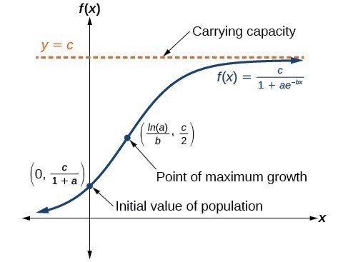
The logistic growth model is approximately exponential at first, but it has a reduced rate of growth as the output approaches the model’s upper bound called the carrying capacity. For constants a, b, and c, the logistic growth of a population over time x is represented by the model
[latex]f\left(x\right)=\dfrac{c}{1+a{e}^{-bx}}[/latex]
The graph below shows how the growth rate changes over time. The graph increases from left to right, but the growth rate only increases until it reaches its point of maximum growth rate at which the rate of increase decreases.
A General Note: Logistic Growth
The logistic growth model is
[latex]f\left(x\right)=\dfrac{c}{1+a{e}^{-bx}}[/latex]
where
- [latex]\dfrac{c}{1+a}[/latex] is the initial value
- [latex]c[/latex] is the carrying capacity or limiting value
- [latex]b[/latex] is a constant determined by the rate of growth.
Example: Using the Logistic-Growth Model
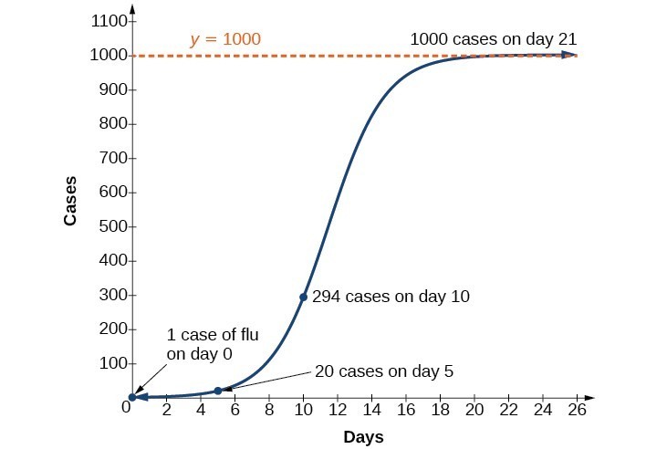
An influenza epidemic spreads through a population rapidly at a rate that depends on two factors. The more people who have the flu, the more rapidly it spreads, and also the more uninfected people there are, the more rapidly it spreads. These two factors make the logistic model good for studying the spread of communicable diseases. And, clearly, there is a maximum value for the number of people infected: the entire population.
For example, at time t = 0 there is one person in a community of 1,000 people who has the flu. So, in that community, at most 1,000 people can have the flu. Researchers find that for this particular strain of the flu, the logistic growth constant is b = 0.6030. Estimate the number of people in this community who will have had this flu after ten days. Predict how many people in this community will have had this flu after a long period of time has passed.
Try It
Using the model in the previous example, estimate the number of cases of flu on day 15.
Choosing an Appropriate Model
Now that we have discussed various mathematical models, we need to learn how to choose the appropriate model for the raw data we have. Many factors influence the choice of a mathematical model among which are experience, scientific laws, and patterns in the data itself. Not all data can be described by elementary functions. Sometimes a function is chosen that approximates the data over a given interval. For instance, suppose data were gathered on the number of homes bought in the United States from the years 1960 to 2013. After plotting these data in a scatter plot, we notice that the shape of the data from the years 2000 to 2013 follow a logarithmic curve. We could restrict the interval from 2000 to 2010, apply regression analysis using a logarithmic model, and use it to predict the number of home buyers for the year 2015.
Three kinds of functions that are often useful in mathematical models are linear functions, exponential functions, and logarithmic functions. If the data lies on a straight line or seems to lie approximately along a straight line, a linear model may be best. If the data is non-linear, we often consider an exponential or logarithmic model although other models, such as quadratic models, may also be considered.
In choosing between an exponential model and a logarithmic model, we look at the way the data curves. This is called the concavity. If we draw a line between two data points, and all (or most) of the data between those two points lies above that line, we say the curve is concave down. We can think of it as a bowl that bends downward and therefore cannot hold water. If all (or most) of the data between those two points lies below the line, we say the curve is concave up. In this case, we can think of a bowl that bends upward and can therefore hold water. An exponential curve, whether rising or falling, whether representing growth or decay, is always concave up away from its horizontal asymptote. A logarithmic curve is always concave down away from its vertical asymptote. In the case of positive data, which is the most common case, an exponential curve is always concave up and a logarithmic curve always concave down.
A logistic curve changes concavity. It starts out concave up and then changes to concave down beyond a certain point, called a point of inflection.
After using the graph to help us choose a type of function to use as a model, we substitute points, and solve to find the parameters. We reduce round-off error by choosing points as far apart as possible.
Example: Choosing a Mathematical Model
Does a linear, exponential, logarithmic, or logistic model best fit the values listed below? Find the model, and use a graph to check your choice.
| x | 1 | 2 | 3 | 4 | 5 | 6 | 7 | 8 | 9 |
| y | 0 | 1.386 | 2.197 | 2.773 | 3.219 | 3.584 | 3.892 | 4.159 | 4.394 |


Try It
Does a linear, exponential, or logarithmic model best fit the data in the table below? Find the model.
| x | 1 | 2 | 3 | 4 | 5 | 6 | 7 | 8 | 9 |
| y | 3.297 | 5.437 | 8.963 | 14.778 | 24.365 | 40.172 | 66.231 | 109.196 | 180.034 |
Expressing an Exponential Model in Base e
While powers and logarithms of any base can be used in modeling, the two most common bases are [latex]10[/latex] and [latex]e[/latex]. In science and mathematics, the base e is often preferred. We can use properties of exponents and properties of logarithms to change any base to base e.
How To: Given a model with the form [latex]y=a{b}^{x}[/latex], change it to the form [latex]y={A}_{0}{e}^{kx}[/latex]
- Rewrite [latex]y=a{b}^{x}[/latex] as [latex]y=a{e}^{\mathrm{ln}\left({b}^{x}\right)}[/latex].
- Use the power rule of logarithms to rewrite as [latex]y=a{e}^{x\mathrm{ln}\left(b\right)}=a{e}^{\mathrm{ln}\left(b\right)x}[/latex].
- Note that [latex]a={A}_{0}[/latex] and [latex]k=\mathrm{ln}\left(b\right)[/latex] in the equation [latex]y={A}_{0}{e}^{kx}[/latex].
Example: Changing to base [latex]e[/latex]
Change the function [latex]y=2.5{\left(3.1\right)}^{x}[/latex] so that this same function is written in the form [latex]y={A}_{0}{e}^{kx}[/latex].
Try It
Change the function [latex]y=3{\left(0.5\right)}^{x}[/latex] to one having e as the base.
Candela Citations
- Revision and Adaptation. Provided by: Lumen Learning. License: CC BY: Attribution
- Question ID 5801. Authored by: Lippman,David. License: CC BY: Attribution. License Terms: IMathAS Community License CC-BY + GPL
- College Algebra. Authored by: Abramson, Jay et al.. Provided by: OpenStax. Located at: http://cnx.org/contents/9b08c294-057f-4201-9f48-5d6ad992740d@5.2. License: CC BY: Attribution. License Terms: Download for free at http://cnx.org/contents/9b08c294-057f-4201-9f48-5d6ad992740d@5.2