Learning Outcomes
- Graph exponential growth and decay functions.
- Solve problems involving radioactive decay, carbon dating, and half life.
Exponential Growth and Decay
tip for success
As you learn about modelling exponential growth and decay, recall familiar techniques that have helped you to model situations using other types of functions. The exponential growth and decay models possess input and corresponding output like other functions graphed in the real plane. They also adhere to the characteristic feature of the graphs of all functions; each point (corresponding input and output pairs) contained on the graph of the function satisfies the equation of the function.
You can rely on these features as you work with the form of the function to fill in known quantities from a given situation to solve for unknowns.
In real-world applications, we need to model the behavior of a function. In mathematical modeling, we choose a familiar general function with properties that suggest that it will model the real-world phenomenon we wish to analyze. In the case of rapid growth, we may choose the exponential growth function:
[latex]y={A}_{0}{e}^{kt}[/latex]
where [latex]{A}_{0}[/latex] is equal to the value at time zero, e is Euler’s constant, and k is a positive constant that determines the rate (percentage) of growth. We may use the exponential growth function in applications involving doubling time, the time it takes for a quantity to double. Such phenomena as wildlife populations, financial investments, biological samples, and natural resources may exhibit growth based on a doubling time. In some applications, however, as we will see when we discuss the logistic equation, the logistic model sometimes fits the data better than the exponential model.
On the other hand, if a quantity is falling rapidly toward zero, without ever reaching zero, then we should probably choose the exponential decay model. Again, we have the form [latex]y={A}_{0}{e}^{-kt}[/latex] where [latex]{A}_{0}[/latex] is the starting value, and e is Euler’s constant. Now k is a negative constant that determines the rate of decay. We may use the exponential decay model when we are calculating half-life, or the time it takes for a substance to exponentially decay to half of its original quantity. We use half-life in applications involving radioactive isotopes.
In our choice of a function to serve as a mathematical model, we often use data points gathered by careful observation and measurement to construct points on a graph and hope we can recognize the shape of the graph. Exponential growth and decay graphs have a distinctive shape, as we can see in the graphs below. It is important to remember that, although parts of each of the two graphs seem to lie on the x-axis, they are really a tiny distance above the x-axis.
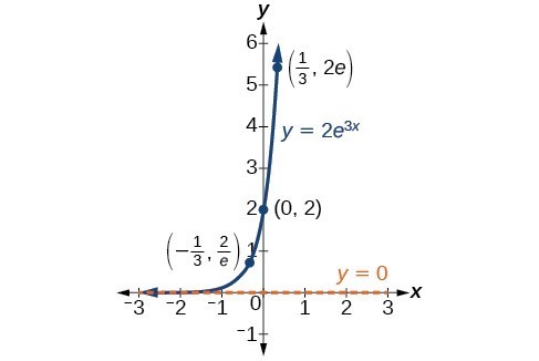
A graph showing exponential growth. The equation is [latex]y=2{e}^{3x}[/latex].
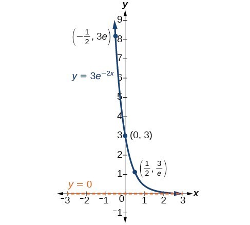
A graph showing exponential decay. The equation is [latex]y=3{e}^{-2x}[/latex].
Exponential growth and decay often involve very large or very small numbers. To describe these numbers, we often use orders of magnitude. The order of magnitude is the power of ten when the number is expressed in scientific notation with one digit to the left of the decimal. For example, the distance to the nearest star, Proxima Centauri, measured in kilometers, is 40,113,497,200,000 kilometers. Expressed in scientific notation, this is [latex]4.01134972\times {10}^{13}[/latex]. We could describe this number as having order of magnitude [latex]{10}^{13}[/latex].
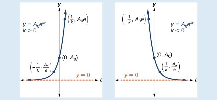
A General Note: Characteristics of the Exponential Function [latex]y=A_{0}e^{kt}[/latex]
An exponential function of the form [latex]y={A}_{0}{e}^{kt}[/latex] has the following characteristics:
- one-to-one function
- horizontal asymptote: y = 0
- domain: [latex]\left(-\infty , \infty \right)[/latex]
- range: [latex]\left(0,\infty \right)[/latex]
- x intercept: none
- y-intercept: [latex]\left(0,{A}_{0}\right)[/latex]
- increasing if k > 0
- decreasing if k < 0
An exponential function models exponential growth when [latex]k > 0[/latex] and exponential decay when [latex]k < 0[/latex].
Try It
The graphs below include important characteristics of an exponential function that can illustrate whether the function represents growth or decay and the speed at which the function grows or decays.
Your task is to add the key features from the graphs above to graph made using an online graphing calculator and adjusting the [latex]a[/latex] and [latex]k[/latex] values. The function [latex]f(x) = a\cdot{e}^{kx}[/latex] will be what you use as your starting point.
Include the following key features:
- The horizontal asymptote
- y-intercept
- The key points labeled in the still graphs above

tip for success
Work through the examples in this section on paper, perhaps more than once or twice, to obtain a thorough understanding of the processes involved.
Example: Graphing Exponential Growth
A population of bacteria doubles every hour. If the culture started with 10 bacteria, graph the population as a function of time.

Calculating Doubling Time
For growing quantities, we might want to find out how long it takes for a quantity to double. As we mentioned above, the time it takes for a quantity to double is called the doubling time.
Given the basic exponential growth equation [latex]A={A}_{0}{e}^{kt}[/latex], doubling time can be found by solving for when the original quantity has doubled, that is, by solving [latex]2{A}_{0}={A}_{0}{e}^{kt}[/latex].
The formula is derived as follows:
[latex]\begin{array}{l}2{A}_{0}={A}_{0}{e}^{kt}\hfill & \hfill \\ 2={e}^{kt}\hfill & \text{Divide both sides by }{A}_{0}.\hfill \\ \mathrm{ln}2=kt\hfill & \text{Take the natural logarithm of both sides}.\hfill \\ t=\frac{\mathrm{ln}2}{k}\hfill & \text{Divide by the coefficient of }t.\hfill \end{array}[/latex]
Thus the doubling time is
[latex]t=\frac{\mathrm{ln}2}{k}[/latex]
Example: Finding a Function That Describes Exponential Growth
According to Moore’s Law, the doubling time for the number of transistors that can be put on a computer chip is approximately two years. Give a function that describes this behavior.
Try It
Recent data suggests that, as of 2013, the rate of growth predicted by Moore’s Law no longer holds. Growth has slowed to a doubling time of approximately three years. Find the new function that takes that longer doubling time into account.
Half-Life
We now turn to exponential decay. One of the common terms associated with exponential decay, as stated above, is half-life, the length of time it takes an exponentially decaying quantity to decrease to half its original amount. Every radioactive isotope has a half-life, and the process describing the exponential decay of an isotope is called radioactive decay.
To find the half-life of a function describing exponential decay, solve the following equation:
[latex]\frac{1}{2}{A}_{0}={A}_{o}{e}^{kt}[/latex]
We find that the half-life depends only on the constant k and not on the starting quantity [latex]{A}_{0}[/latex].
The formula is derived as follows
[latex]\begin{array}{l}\frac{1}{2}{A}_{0}={A}_{o}{e}^{kt}\hfill & \hfill \\ \frac{1}{2}={e}^{kt}\hfill & \text{Divide both sides by }{A}_{0}.\hfill \\ \mathrm{ln}\left(\frac{1}{2}\right)=kt\hfill & \text{Take the natural log of both sides}.\hfill \\ -\mathrm{ln}\left(2\right)=kt\hfill & \text{Apply properties of logarithms}.\hfill \\ -\frac{\mathrm{ln}\left(2\right)}{k}=t\hfill & \text{Divide by }k.\hfill \end{array}[/latex]
Since t, the time, is positive, k must, as expected, be negative. This gives us the half-life formula
[latex]t=-\frac{\mathrm{ln}\left(2\right)}{k}[/latex]
In previous sections, we learned the properties and rules for both exponential and logarithmic functions. We have seen that any exponential function can be written as a logarithmic function and vice versa. We have used exponents to solve logarithmic equations and logarithms to solve exponential equations. We are now ready to combine our skills to solve equations that model real-world situations, whether the unknown is in an exponent or in the argument of a logarithm.
tip for success
As you learn to model real-world applications using exponential and logarithmic functions, it will be helpful to have created a reference list of the properties and rules for exponents and logarithms as well as the techniques for solving exponential and logarithmic equations. Keep this reference list nearby as you practice working through the examples. Eventually, you’ll be able to work through new applications without referring to your notes.
The applications below use exponential and logarithmic functions to model behavior in the real world.
One such application is in science, in calculating the time it takes for half of the unstable material in a sample of a radioactive substance to decay, called its half-life. The table below lists the half-life for several of the more common radioactive substances.
| Substance | Use | Half-life |
|---|---|---|
| gallium-67 | nuclear medicine | 80 hours |
| cobalt-60 | manufacturing | 5.3 years |
| technetium-99m | nuclear medicine | 6 hours |
| americium-241 | construction | 432 years |
| carbon-14 | archeological dating | 5,715 years |
| uranium-235 | atomic power | 703,800,000 years |
We can see how widely the half-lives for these substances vary. Knowing the half-life of a substance allows us to calculate the amount remaining after a specified time. We can use the formula for radioactive decay:
[latex]\begin{array}{l}A\left(t\right)={A}_{0}{e}^{\frac{\mathrm{ln}\left(0.5\right)}{T}t}\hfill \\ A\left(t\right)={A}_{0}{e}^{\mathrm{ln}\left(0.5\right)\frac{t}{T}}\hfill \\ A\left(t\right)={A}_{0}{\left({e}^{\mathrm{ln}\left(0.5\right)}\right)}^{\frac{t}{T}}\hfill \\ A\left(t\right)={A}_{0}{\left(\frac{1}{2}\right)}^{\frac{t}{T}}\hfill \end{array}[/latex]
where
- [latex]{A}_{0}[/latex] is the amount initially present
- [latex]T[/latex] is the half-life of the substance
- [latex]t[/latex] is the time period over which the substance is studied
- [latex]A[/latex], or [latex]A(t)[/latex], is the amount of the substance present after time [latex]t[/latex]
How To: Given the half-life, find the decay rate
- Write [latex]A={A}_{o}{e}^{kt}[/latex].
- Replace A by [latex]\frac{1}{2}{A}_{0}[/latex] and replace t by the given half-life.
- Solve to find k. Express k as an exact value (do not round).
Note: It is also possible to find the decay rate using [latex]k=-\frac{\mathrm{ln}\left(2\right)}{t}[/latex].
Example: Using the Formula for Radioactive Decay to Find the Quantity of a Substance
How long will it take for 10% of a 1000-gram sample of uranium-235 to decay?
Try It
How long will it take before twenty percent of our 1000-gram sample of uranium-235 has decayed?
Example: Finding the Function that Describes Radioactive Decay
The half-life of carbon-14 is 5,730 years. Express the amount of carbon-14 remaining as a function of time, t.
Try It
The half-life of plutonium-244 is 80,000,000 years. Find a function that gives the amount of plutonium-244 remaining as a function of time measured in years.
Radiocarbon Dating
The formula for radioactive decay is important in radiocarbon dating which is used to calculate the approximate date a plant or animal died. Radiocarbon dating was discovered in 1949 by Willard Libby who won a Nobel Prize for his discovery. It compares the difference between the ratio of two isotopes of carbon in an organic artifact or fossil to the ratio of those two isotopes in the air. It is believed to be accurate to within about 1% error for plants or animals that died within the last 60,000 years.
Carbon-14 is a radioactive isotope of carbon that has a half-life of 5,730 years. It occurs in small quantities in the carbon dioxide in the air we breathe. Most of the carbon on Earth is carbon-12 which has an atomic weight of 12 and is not radioactive. Scientists have determined the ratio of carbon-14 to carbon-12 in the air for the last 60,000 years using tree rings and other organic samples of known dates—although the ratio has changed slightly over the centuries.
As long as a plant or animal is alive, the ratio of the two isotopes of carbon in its body is close to the ratio in the atmosphere. When it dies, the carbon-14 in its body decays and is not replaced. By comparing the ratio of carbon-14 to carbon-12 in a decaying sample to the known ratio in the atmosphere, the date the plant or animal died can be approximated.
Since the half-life of carbon-14 is 5,730 years, the formula for the amount of carbon-14 remaining after t years is
[latex]A\approx {A}_{0}{e}^{\left(\frac{\mathrm{ln}\left(0.5\right)}{5730}\right)t}[/latex]
where
- [latex]A[/latex] is the amount of carbon-14 remaining
- [latex]{A}_{0}[/latex] is the amount of carbon-14 when the plant or animal began decaying.
This formula is derived as follows:
[latex]\begin{array}{l}\text{ }A={A}_{0}{e}^{kt}\hfill & \text{The continuous growth formula}.\hfill \\ \text{ }0.5{A}_{0}={A}_{0}{e}^{k\cdot 5730}\hfill & \text{Substitute the half-life for }t\text{ and }0.5{A}_{0}\text{ for }f\left(t\right).\hfill \\ \text{ }0.5={e}^{5730k}\hfill & \text{Divide both sides by }{A}_{0}.\hfill \\ \mathrm{ln}\left(0.5\right)=5730k\hfill & \text{Take the natural log of both sides}.\hfill \\ \text{ }k=\frac{\mathrm{ln}\left(0.5\right)}{5730}\hfill & \text{Divide both sides by the coefficient of }k.\hfill \\ \text{ }A={A}_{0}{e}^{\left(\frac{\mathrm{ln}\left(0.5\right)}{5730}\right)t}\hfill & \text{Substitute for }r\text{ in the continuous growth formula}.\hfill \end{array}[/latex]
To find the age of an object we solve this equation for t:
[latex]t=\frac{\mathrm{ln}\left(\frac{A}{{A}_{0}}\right)}{-0.000121}[/latex]
Out of necessity, we neglect here the many details that a scientist takes into consideration when doing carbon-14 dating, and we only look at the basic formula. The ratio of carbon-14 to carbon-12 in the atmosphere is approximately 0.0000000001%. Let r be the ratio of carbon-14 to carbon-12 in the organic artifact or fossil to be dated determined by a method called liquid scintillation. From the equation [latex]A\approx {A}_{0}{e}^{-0.000121t}[/latex] we know the ratio of the percentage of carbon-14 in the object we are dating to the percentage of carbon-14 in the atmosphere is [latex]r=\frac{A}{{A}_{0}}\approx {e}^{-0.000121t}[/latex]. We solve this equation for t, to get
[latex]t=\frac{\mathrm{ln}\left(r\right)}{-0.000121}[/latex]
How To: Given the percentage of carbon-14 in an object, determine its age
- Express the given percentage of carbon-14 as an equivalent decimal r.
- Substitute for r in the equation [latex]t=\frac{\mathrm{ln}\left(r\right)}{-0.000121}[/latex] and solve for the age, t.
Example: Finding the Age of a Bone
A bone fragment is found that contains 20% of its original carbon-14. To the nearest year, how old is the bone?
Try It
Cesium-137 has a half-life of about 30 years. If we begin with 200 mg of cesium-137, will it take more or less than 230 years until only 1 milligram remains?
Candela Citations
- Revision and Adaptation. Provided by: Lumen Learning. License: CC BY: Attribution
- Exponential Growth and Decay Interactive. Authored by: Lumen Learning. Located at: https://www.desmos.com/calculator/4zae7vnjfr. License: Public Domain: No Known Copyright
- Question ID 29686. Authored by: McClure,Caren. License: CC BY: Attribution. License Terms: IMathAS Community License CC-BY + GPL
- College Algebra. Authored by: Abramson, Jay et al.. Provided by: OpenStax. Located at: http://cnx.org/contents/9b08c294-057f-4201-9f48-5d6ad992740d@5.2. License: CC BY: Attribution. License Terms: Download for free at http://cnx.org/contents/9b08c294-057f-4201-9f48-5d6ad992740d@5.2
- Question ID 100026. Authored by: Rieman,Rick. License: CC BY: Attribution. License Terms: IMathAS Community License CC-BY + GPL