Learning Outcomes
- Determine whether an exponential function and its associated graph represents growth or decay.
- Sketch a graph of an exponential function.
Before we begin graphing, it is helpful to review the behavior of exponential growth. Recall the table of values for a function of the form [latex]f\left(x\right)={b}^{x}[/latex] whose base is greater than one. We’ll use the function [latex]f\left(x\right)={2}^{x}[/latex]. Observe how the output values in the table below change as the input increases by 1.
| x | –3 | –2 | –1 | 0 | 1 | 2 | 3 |
| [latex]f\left(x\right)={2}^{x}[/latex] | [latex]\frac{1}{8}[/latex] | [latex]\frac{1}{4}[/latex] | [latex]\frac{1}{2}[/latex] | 1 | 2 | 4 | 8 |
Each output value is the product of the previous output and the base, 2. We call the base 2 the constant ratio. In fact, for any exponential function with the form [latex]f\left(x\right)=a{b}^{x}[/latex], b is the constant ratio of the function. This means that as the input increases by 1, the output value will be the product of the base and the previous output, regardless of the value of a.
Notice from the table that:
- the output values are positive for all values of x
- as x increases, the output values increase without bound
- as x decreases, the output values grow smaller, approaching zero
The graph below shows the exponential growth function [latex]f\left(x\right)={2}^{x}[/latex].
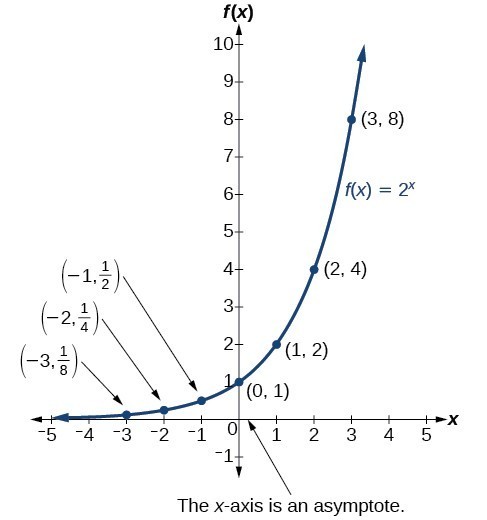
Notice that the graph gets close to the x-axis but never touches it.
The domain of [latex]f\left(x\right)={2}^{x}[/latex] is all real numbers, the range is [latex]\left(0,\infty \right)[/latex], and the horizontal asymptote is [latex]y=0[/latex].
To get a sense of the behavior of exponential decay, we can create a table of values for a function of the form [latex]f\left(x\right)={b}^{x}[/latex] whose base is between zero and one. We’ll use the function [latex]g\left(x\right)={\left(\frac{1}{2}\right)}^{x}[/latex]. Observe how the output values in the table below change as the input increases by 1.
| x | –3 | –2 | –1 | 0 | 1 | 2 | 3 |
| [latex]g\left(x\right)=\left(\frac{1}{2}\right)^{x}[/latex] | 8 | 4 | 2 | 1 | [latex]\frac{1}{2}[/latex] | [latex]\frac{1}{4}[/latex] | [latex]\frac{1}{8}[/latex] |
Again, because the input is increasing by 1, each output value is the product of the previous output and the base or constant ratio [latex]\frac{1}{2}[/latex].
Notice from the table that:
- the output values are positive for all values of x
- as x increases, the output values grow smaller, approaching zero
- as x decreases, the output values grow without bound
The graph below shows the exponential decay function, [latex]g\left(x\right)={\left(\frac{1}{2}\right)}^{x}[/latex].
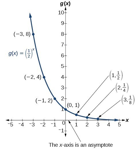
The domain of [latex]g\left(x\right)={\left(\frac{1}{2}\right)}^{x}[/latex] is all real numbers, the range is [latex]\left(0,\infty \right)[/latex], and the horizontal asymptote is [latex]y=0[/latex].
A General Note: Characteristics of the Graph of the Parent Function [latex]f\left(x\right)={b}^{x}[/latex]
An exponential function with the form [latex]f\left(x\right)={b}^{x}[/latex], [latex]b>0[/latex], [latex]b\ne 1[/latex], has these characteristics:
- one-to-one function
- horizontal asymptote: [latex]y=0[/latex]
- domain: [latex]\left(-\infty , \infty \right)[/latex]
- range: [latex]\left(0,\infty \right)[/latex]
- x-intercept: none
- y-intercept: [latex]\left(0,1\right)[/latex]
- increasing if [latex]b>1[/latex]
- decreasing if [latex]b<1[/latex]
Use an online graphing tool to graph [latex]f\left(x\right)={b}^{x}[/latex].
Adjust the [latex]b[/latex] values to see various graphs of exponential growth and decay functions.
Try decimal values between [latex]0[/latex] and [latex]1[/latex], and also values greater than [latex]1[/latex]. Which one is growth and which one is decay?
How To: Given an exponential function of the form [latex]f\left(x\right)={b}^{x}[/latex], graph the function
- Create a table of points.
- Plot at least 3 point from the table including the y-intercept [latex]\left(0,1\right)[/latex].
- Draw a smooth curve through the points.
- State the domain, [latex]\left(-\infty ,\infty \right)[/latex], the range, [latex]\left(0,\infty \right)[/latex], and the horizontal asymptote, [latex]y=0[/latex].
tip for success
When sketching the graph of an exponential function by plotting points, include a few input values left and right of zero as well as zero itself.
With few exceptions, such as functions that would be undefined at zero or negative input like the radical or (as you’ll see soon) the logarithmic function, it is good practice to let the input equal [latex]-3, -2, -1, 0, 1, 2, \text{ and } 3[/latex] to get the idea of the shape of the graph.
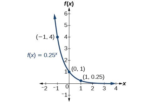
Example: Sketching the Graph of an Exponential Function of the Form [latex]f\left(x\right)={b}^{x}[/latex]
Sketch a graph of [latex]f\left(x\right)={0.25}^{x}[/latex]. State the domain, range, and asymptote.
Watch the following video for another example of graphing an exponential function. The base of the exponential term is between [latex]0[/latex] and [latex]1[/latex], so this graph will represent decay.
The next example shows how to plot an exponential growth function where the base is greater than [latex]1[/latex].
Example
Sketch a graph of [latex]f(x)={\sqrt{2}(\sqrt{2})}^{x}[/latex]. State the domain and range.
The next video example includes graphing an exponential growth function and defining the domain and range of the function.
Try It
Sketch the graph of [latex]f\left(x\right)={4}^{x}[/latex]. State the domain, range, and asymptote.

Candela Citations
- Revision and Adaptation. Provided by: Lumen Learning. License: CC BY: Attribution
- Characteristics of Graphs of Exponential Functions Interactive. Authored by: Lumen Learning. Located at: https://www.desmos.com/calculator/3pqyjsunkg. License: Public Domain: No Known Copyright
- Graph a Basic Exponential Function Using a Table of Values. Authored by: James Sousa (Mathispower4u.com) for Lumen Learning. Located at: https://youtu.be/FMzZB9Ve-1U. License: CC BY: Attribution
- Graph an Exponential Function Using a Table of Values. Authored by: James Sousa (Mathispower4u.com) for Lumen Learning. Located at: https://youtu.be/M6bpp0BRIf0. License: CC BY: Attribution
- Question ID 3607. Authored by: Jay Abramson, et al.. Provided by: Reidel,Jessica. License: CC BY: Attribution. License Terms: IMathAS Community License CC-BY + GPL
- College Algebra. Authored by: Abramson, Jay et al.. Provided by: OpenStax. Located at: http://cnx.org/contents/9b08c294-057f-4201-9f48-5d6ad992740d@5.2. License: CC BY: Attribution. License Terms: Download for free at http://cnx.org/contents/9b08c294-057f-4201-9f48-5d6ad992740d@5.2
- Precalculus. Authored by: Jay Abramson, et al.. Provided by: OpenStax. Located at: http://cnx.org/contents/fd53eae1-fa23-47c7-bb1b-972349835c3c@5.175. License: CC BY: Attribution. License Terms: Download For Free at : http://cnx.org/contents/fd53eae1-fa23-47c7-bb1b-972349835c3c@5.175.