Learning Outcomes
- Graph exponential functions shifted horizontally or vertically and write the associated equation.
Transformations of exponential graphs behave similarly to those of other functions. Just as with other parent functions, we can apply the four types of transformations—shifts, reflections, stretches, and compressions—to the parent function [latex]f\left(x\right)={b}^{x}[/latex] without loss of shape. For instance, just as the quadratic function maintains its parabolic shape when shifted, reflected, stretched, or compressed, the exponential function also maintains its general shape regardless of the transformations applied.
Tip for success
Translating exponential functions follows the same ideas you’ve used to translate other functions. Add or subtract a value inside the function argument (in the exponent) to shift horizontally, and add or subtract a value outside the function argument to shift vertically.
Graphing a Vertical Shift
The first transformation occurs when we add a constant d to the parent function [latex]f\left(x\right)={b}^{x}[/latex] giving us a vertical shift d units in the same direction as the sign. For example, if we begin by graphing a parent function, [latex]f\left(x\right)={2}^{x}[/latex], we can then graph two vertical shifts alongside it using [latex]d=3[/latex]: the upward shift, [latex]g\left(x\right)={2}^{x}+3[/latex] and the downward shift, [latex]h\left(x\right)={2}^{x}-3[/latex]. Both vertical shifts are shown in the figure below.
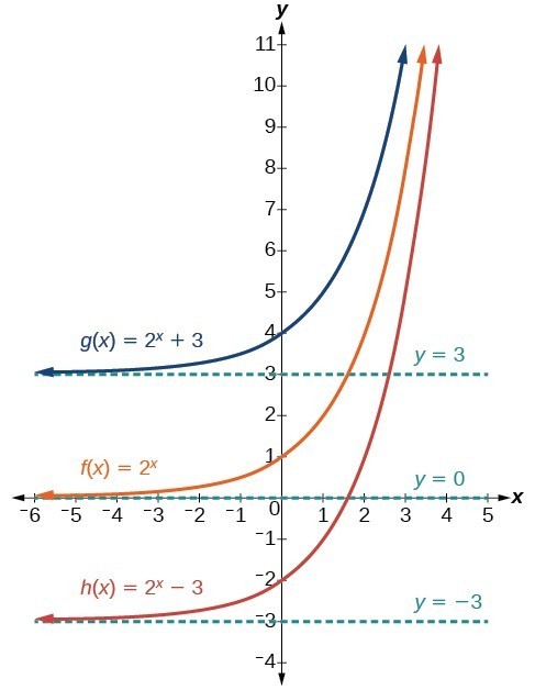
Observe the results of shifting [latex]f\left(x\right)={2}^{x}[/latex] vertically:
- The domain [latex]\left(-\infty ,\infty \right)[/latex] remains unchanged.
- When the function is shifted up 3 units giving [latex]g\left(x\right)={2}^{x}+3[/latex]:
- The y-intercept shifts up 3 units to [latex]\left(0,4\right)[/latex].
- The asymptote shifts up 3 units to [latex]y=3[/latex].
- The range becomes [latex]\left(3,\infty \right)[/latex].
- When the function is shifted down 3 units giving [latex]h\left(x\right)={2}^{x}-3[/latex]:
- The y-intercept shifts down 3 units to [latex]\left(0,-2\right)[/latex].
- The asymptote also shifts down 3 units to [latex]y=-3[/latex].
- The range becomes [latex]\left(-3,\infty \right)[/latex].
Try it
- Use an online graphing calculator to plot [latex]f(x) = 2^x+a[/latex]
- Adjust the value of [latex]a[/latex] until the graph has been shifted 4 units up.
- Add a line that represents the horizontal asymptote for this function. What is the equation for this function? What is the new y-intercept? What is its domain and range?
- Now create a graph of the function [latex]f(x) = 2^x[/latex] that has been shifted down 2 units. Add a line that represents the horizontal asymptote. What is the equation for this function? What is the new y-intercept? What is its domain and range?
Graphing a Horizontal Shift
The next transformation occurs when we add a constant c to the input of the parent function [latex]f\left(x\right)={b}^{x}[/latex] giving us a horizontal shift c units in the opposite direction of the sign. For example, if we begin by graphing the parent function [latex]f\left(x\right)={2}^{x}[/latex], we can then graph two horizontal shifts alongside it using [latex]c=3[/latex]: the shift left, [latex]g\left(x\right)={2}^{x+3}[/latex], and the shift right, [latex]h\left(x\right)={2}^{x - 3}[/latex]. Both horizontal shifts are shown in the graph below.
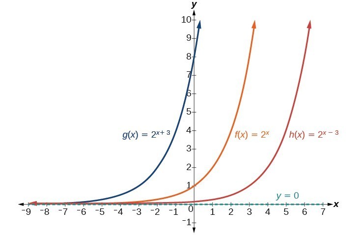
Observe the results of shifting [latex]f\left(x\right)={2}^{x}[/latex] horizontally:
- The domain, [latex]\left(-\infty ,\infty \right)[/latex], remains unchanged.
- The asymptote, [latex]y=0[/latex], remains unchanged.
- The y-intercept shifts such that:
- When the function is shifted left 3 units to [latex]g\left(x\right)={2}^{x+3}[/latex], the y-intercept becomes [latex]\left(0,8\right)[/latex]. This is because [latex]{2}^{x+3}=\left({2}^{3}\right){2}^{x}=\left(8\right){2}^{x}[/latex], so the initial value of the function is 8.
- When the function is shifted right 3 units to [latex]h\left(x\right)={2}^{x - 3}[/latex], the y-intercept becomes [latex]\left(0,\frac{1}{8}\right)[/latex]. Again, see that [latex]{2}^{x-3}=\left({2}^{-3}\right){2}^{x}=\left(\frac{1}{8}\right){2}^{x}[/latex], so the initial value of the function is [latex]\frac{1}{8}[/latex].
try it
- Using an online graphing calculator, plot [latex]f(x) = 2^{(x+a)}[/latex]
- Adjust the value of [latex]a[/latex] until the graph is shifted 4 units to the right. What is the equation for this function? What is the new y-intercept? What are its domain and range?
- Now adjust the value of [latex]a[/latex] until the graph has been shifted 3 units to the left. What is the equation for this function? What is the new y-intercept? What are its domain and range?
A General Note: Shifts of the Parent Function [latex]f\left(x\right)={b}^{x}[/latex]
For any constants c and d, the function [latex]f\left(x\right)={b}^{x+c}+d[/latex] shifts the parent function [latex]f\left(x\right)={b}^{x}[/latex]
- shifts the parent function [latex]f\left(x\right)={b}^{x}[/latex] vertically d units, in the same direction as the sign of d.
- shifts the parent function [latex]f\left(x\right)={b}^{x}[/latex] horizontally c units, in the opposite direction as the sign of c.
- has a y-intercept of [latex]\left(0,{b}^{c}+d\right)[/latex].
- has a horizontal asymptote of y = d.
- has a range of [latex]\left(d,\infty \right)[/latex].
- has a domain of [latex]\left(-\infty ,\infty \right)[/latex] which remains unchanged.
How To: Given an exponential function with the form [latex]f\left(x\right)={b}^{x+c}+d[/latex], graph the translation
- Draw the horizontal asymptote y = d.
- Shift the graph of [latex]f\left(x\right)={b}^{x}[/latex] left c units if c is positive and right [latex]c[/latex] units if c is negative.
- Shift the graph of [latex]f\left(x\right)={b}^{x}[/latex] up d units if d is positive and down d units if d is negative.
- State the domain, [latex]\left(-\infty ,\infty \right)[/latex], the range, [latex]\left(d,\infty \right)[/latex], and the horizontal asymptote [latex]y=d[/latex].
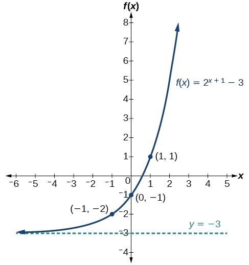
Example: Graphing a Shift of an Exponential Function
Graph [latex]f\left(x\right)={2}^{x+1}-3[/latex]. State the domain, range, and asymptote.
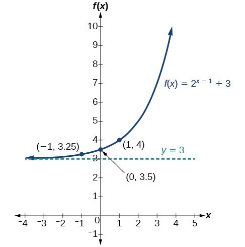
Try It
Use an online graphing calculator to plot the function [latex]f\left(x\right)={2}^{x-1}+3[/latex]. State domain, range, and asymptote.
Watch the following video for more examples of the difference between horizontal and vertical shifts of exponential functions and the resulting graphs and equations.
Using a Graph to Approximate a Solution to an Exponential Equation
Graphing can help you confirm or find the solution to an exponential equation. An exponential equation is different from a function because a function is a large collection of points made of inputs and corresponding outputs, whereas equations that you have seen typically have one, two, or no solutions. For example, [latex]f(x)=2^{x}[/latex] is a function and is comprised of many points [latex](x,f(x))[/latex], and [latex]4=2^{x}[/latex] can be solved to find the specific value for x that makes it a true statement. The graph below shows the intersection of the line [latex]f(x)=4[/latex] and [latex]f(x)=2^{x}[/latex]. You can see they cross at [latex]y=4[/latex].

In the following example you can try this yourself.
Example : Approximating the Solution of an Exponential Equation
Use an online graphing calculator to solve [latex]42=1.2{\left(5\right)}^{x}+2.8[/latex] graphically.
Try It
Solve [latex]4=7.85{\left(1.15\right)}^{x}-2.27[/latex] graphically. Round to the nearest thousandth.
Candela Citations
- Revision and Adaptation. Provided by: Lumen Learning. License: CC BY: Attribution
- Horizontal and Vertical Translations of Exponential Functions Interactive. Authored by: Lumen Learning. Located at: https://www.desmos.com/calculator/5mrjqegkxk. License: Public Domain: No Known Copyright
- Horizontal and Vertical Translations of Exponential Functions 2 Interactive. Authored by: Lumen Learning. Located at: https://www.desmos.com/calculator/rpv1kea0pz. License: Public Domain: No Known Copyright
- Horizontal and Vertical Translations of Exponential Functions 3 Interactive. Authored by: Lumen Learning. Located at: https://www.desmos.com/calculator/e5l4eca3ob. License: Public Domain: No Known Copyright
- Solve Exponential Interactive. Authored by: Lumen Learning. Located at: https://www.desmos.com/calculator/lhmpdkbjt0. License: Public Domain: No Known Copyright
- Horizontal and Vertical Translations of Exponential Functions 4 Interactive. Authored by: Lumen Learning. Located at: https://www.desmos.com/calculator/ozaejvejqn. License: Public Domain: No Known Copyright
- College Algebra. Authored by: Abramson, Jay et al.. Provided by: OpenStax. Located at: http://cnx.org/contents/9b08c294-057f-4201-9f48-5d6ad992740d@5.2. License: CC BY: Attribution. License Terms: Download for free at http://cnx.org/contents/9b08c294-057f-4201-9f48-5d6ad992740d@5.2
- Question ID 63064. Authored by: Brin,Leon. License: CC BY: Attribution. License Terms: IMathAS Community License CC-BY + GPL
- Ex: Match the Graphs of Translated Exponential Function to Equations. Authored by: James Sousa (Mathispower4u.com). Located at: https://youtu.be/phYxEeJ7ZW4. License: CC BY: Attribution