Learning Outcomes
- Determine whether data or a scenario describe linear or geometric growth
- Identify growth rates, initial values, or point values expressed verbally, graphically, or numerically, and translate them into a format usable in calculation
- Calculate recursive and explicit equations for linear and geometric growth given sufficient information, and use those equations to make predictions
Population Growth
Suppose that every year, only 10% of the fish in a lake have surviving offspring. If there were 100 fish in the lake last year, there would now be 110 fish. If there were 1000 fish in the lake last year, there would now be 1100 fish. Absent any inhibiting factors, populations of people and animals tend to grow by a percent of the existing population each year.

Suppose our lake began with 1000 fish, and 10% of the fish have surviving offspring each year. Since we start with 1000 fish, P0 = 1000. How do we calculate P1? The new population will be the old population, plus an additional 10%. Symbolically:
P1 = P0 + 0.10P0
Notice this could be condensed to a shorter form by factoring:
P1 = P0 + 0.10P0 = 1P0 + 0.10P0 = (1+ 0.10)P0 = 1.10P0
While 10% is the growth rate, 1.10 is the growth multiplier. Notice that 1.10 can be thought of as “the original 100% plus an additional 10%.”
For our fish population,
P1 = 1.10(1000) = 1100
We could then calculate the population in later years:
P2 = 1.10P1 = 1.10(1100) = 1210
P3 = 1.10P2 = 1.10(1210) = 1331
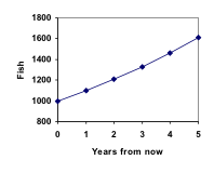
Notice that in the first year, the population grew by 100 fish; in the second year, the population grew by 110 fish; and in the third year the population grew by 121 fish.
While there is a constant percentage growth, the actual increase in number of fish is increasing each year.
Graphing these values we see that this growth doesn’t quite appear linear.
A walkthrough of this fish scenario can be viewed here:
To get a better picture of how this percentage-based growth affects things, we need an explicit form, so we can quickly calculate values further out in the future.
Like we did for the linear model, we will start building from the recursive equation:
P1 = 1.10P0 = 1.10(1000)
P2 = 1.10P1 = 1.10(1.10(1000)) = 1.102(1000)
P3 = 1.10P2 = 1.10(1.102(1000)) = 1.103(1000)
P4 = 1.10P3 = 1.10(1.103(1000)) = 1.104(1000)
Observing a pattern, we can generalize the explicit form to be:
Pn = 1.10n(1000), or equivalently, Pn = 1000(1.10n)
From this, we can quickly calculate the number of fish in 10, 20, or 30 years:
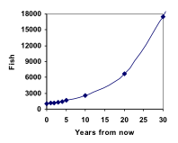
P10 = 1.1010(1000) = 2594
P20 = 1.1020(1000) = 6727
P30 = 1.1030(1000) = 17449
Adding these values to our graph reveals a shape that is definitely not linear. If our fish population had been growing linearly, by 100 fish each year, the population would have only reached 4000 in 30 years, compared to almost 18,000 with this percent-based growth, called exponential growth.
A video demonstrating the explicit model of this fish story can be viewed here:
In exponential growth, the population grows proportional to the size of the population, so as the population gets larger, the same percent growth will yield a larger numeric growth.
Exponential Growth
If a quantity starts at size P0 and grows by R% (written as a decimal, r) every time period, then the quantity after n time periods can be determined using either of these relations:
Recursive form
Pn = (1+r) Pn-1
Explicit form
Pn = (1+r)n P0 or equivalently, Pn = P0 (1+r)n
We call r the growth rate.
The term (1+r) is called the growth multiplier, or common ratio.
Example
Between 2007 and 2008, Olympia, WA grew almost 3% to a population of 245 thousand people. If this growth rate was to continue, what would the population of Olympia be in 2014?
The following video explains this example in detail.
Evaluating exponents on the calculator
To evaluate expressions like (1.03)6, it will be easier to use a calculator than multiply 1.03 by itself six times. Most scientific calculators have a button for exponents. It is typically either labeled like:
^ , yx , or xy .
To evaluate 1.036 we’d type 1.03 ^ 6, or 1.03 yx 6. Try it out – you should get an answer around 1.1940523.
Try It
India is the second most populous country in the world, with a population in 2008 of about 1.14 billion people. The population is growing by about 1.34% each year. If this trend continues, what will India’s population grow to by 2020?
Examples
A friend is using the equation Pn = 4600(1.072)n to predict the annual tuition at a local college. She says the formula is based on years after 2010. What does this equation tell us?
View the following to see this example worked out.
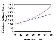
In 1990, residential energy use in the US was responsible for 962 million metric tons of carbon dioxide emissions. By the year 2000, that number had risen to 1182 million metric tons[1]. If the emissions grow exponentially and continue at the same rate, what will the emissions grow to by 2050?
View more about this example here.
Rounding
As a note on rounding, notice that if we had rounded the growth rate to 2.1%, our calculation for the emissions in 2050 would have been 3347. Rounding to 2% would have changed our result to 3156. A very small difference in the growth rates gets magnified greatly in exponential growth. For this reason, it is recommended to round the growth rate as little as possible.
If you need to round, keep at least three significant digits – numbers after any leading zeros. So 0.4162 could be reasonably rounded to 0.416. A growth rate of 0.001027 could be reasonably rounded to 0.00103.
Evaluating roots on the calculator
In the previous example, we had to calculate the 10th root of a number. This is different than taking the basic square root, √. Many scientific calculators have a button for general roots. It is typically labeled like:
[latex]\sqrt[y]{x}[/latex]
To evaluate the 3rd root of 8, for example, we’d either type 3 [latex]\sqrt[x]{{}}[/latex] 8, or 8 [latex]\sqrt[x]{{}}[/latex] 3, depending on the calculator. Try it on yours to see which to use – you should get an answer of 2.
If your calculator does not have a general root button, all is not lost. You can instead use the property of exponents which states that:
[latex]\sqrt[n]{a}={a}^{\frac{1}{2}}[/latex].
So, to compute the 3rd root of 8, you could use your calculator’s exponent key to evaluate 81/3. To do this, type:
8 yx ( 1 ÷ 3 )
The parentheses tell the calculator to divide 1/3 before doing the exponent.
Try It
The number of users on a social networking site was 45 thousand in February when they officially went public, and grew to 60 thousand by October. If the site is growing exponentially, and growth continues at the same rate, how many users should they expect two years after they went public?
Example
Looking back at the last example, for the sake of comparison, what would the carbon emissions be in 2050 if emissions grow linearly at the same rate?
A demonstration of this example can be seen in the following video.
So how do we know which growth model to use when working with data? There are two approaches which should be used together whenever possible:
- Find more than two pieces of data. Plot the values, and look for a trend. Does the data appear to be changing like a line, or do the values appear to be curving upwards?
- Consider the factors contributing to the data. Are they things you would expect to change linearly or exponentially? For example, in the case of carbon emissions, we could expect that, absent other factors, they would be tied closely to population values, which tend to change exponentially.
Candela Citations
- Revision and Adaptation. Provided by: Lumen Learning. License: CC BY: Attribution
- Exponential (Geometric) Growth. Authored by: David Lippman. Located at: http://www.opentextbookstore.com/mathinsociety/. Project: Math in Society. License: CC BY-SA: Attribution-ShareAlike
- calf-fish-lake-pond-river. Authored by: Pexels. Located at: https://pixabay.com/en/calf-fish-lake-pond-river-1869984/. License: CC0: No Rights Reserved
- Exponential Growth Model Part 1. Authored by: OCLPhase2's channel. Located at: https://youtu.be/3BiU7Ihxvxg. License: CC BY: Attribution
- Exponential Growth Model Part 2. Authored by: OCLPhase2's channel. Located at: https://youtu.be/tg2ysaZ8agY. License: CC BY: Attribution
- Predicting future population using an exponential model. Authored by: OCLPhase2's channel. Located at: https://youtu.be/CDI4xS65rxY. License: CC BY: Attribution
- Interpreting an Exponential Equation. Authored by: OCLPhase2's channel. Located at: https://youtu.be/T8Yz94De5UM. License: CC BY: Attribution
- Finding an Exponential Model. Authored by: OCLPhase2's channel. Located at: https://youtu.be/9Zu2uONfLkQ. License: CC BY: Attribution
- Comparing exponential to linear growth. Authored by: OCLPhase2's channel. Located at: https://youtu.be/yiuZoiRMtYM. License: CC BY: Attribution
- Question ID 6598. Authored by: Lippman, David. License: CC BY: Attribution. License Terms: IMathAS Community License CC-BY + GPL