Learning Objectives
- Create and apply conditional formatting.
As we have learned so far, Excel has a wide variety of easy to use tools for organizing, sorting, and otherwise marking information. Think back to when we applied styles to a cell to indicate good information or information that needs to be verified. Excel also has the ability to automatically apply such markings through conditional formatting.
With conditional formatting, you provide Excel with a rule, such as “less than 10,” and the program will scan through your data and highlight all the cells that meet that rule. There are several rules already available, but you can also create and apply your own rules and visual clues.
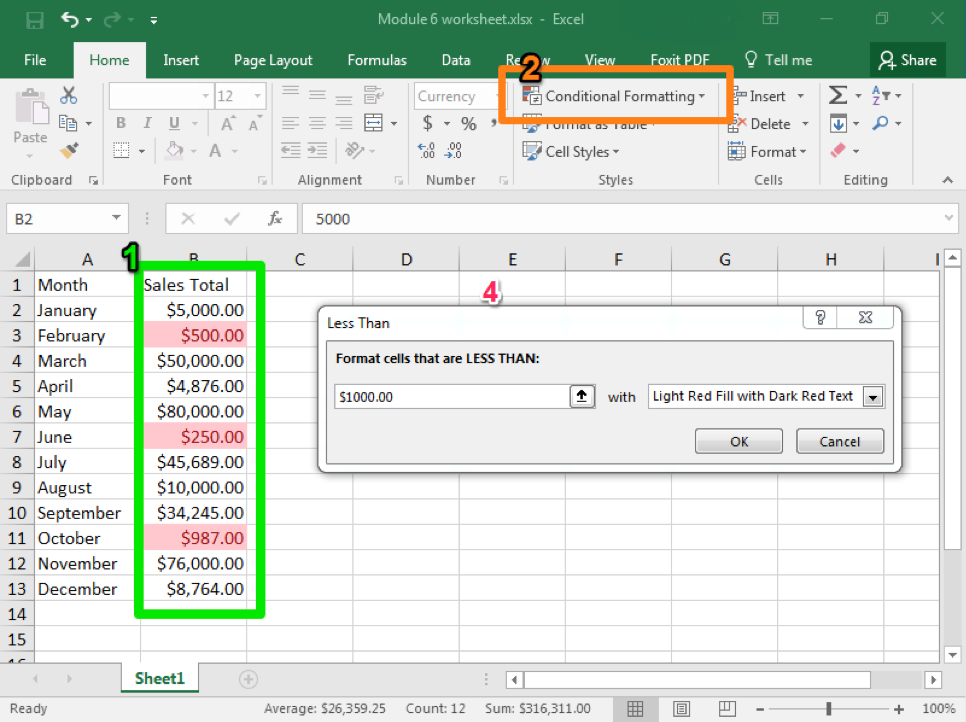
- Select the cells, rows, or columns you wish to have conditional formatting.
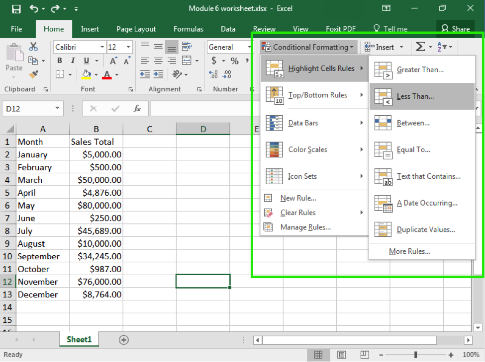
- From the Styles group, click on the Conditional Formatting button
- Select the style of formatting you would like. Here we have Highlight Cell Rules.
- Select the specific type of rule you would like to use and then apply your target value. Here we have selected Less Than.
- The formatting will appear automatically so you can see what it will look like. Note that Excel will automatically provide a value, but you can manually change it.
- Hit OK if you wish to apply the formatting. Otherwise, when you leave the formatting menu, it will disappear.
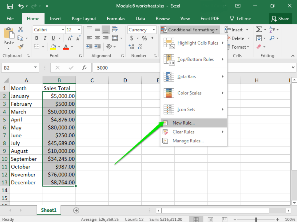
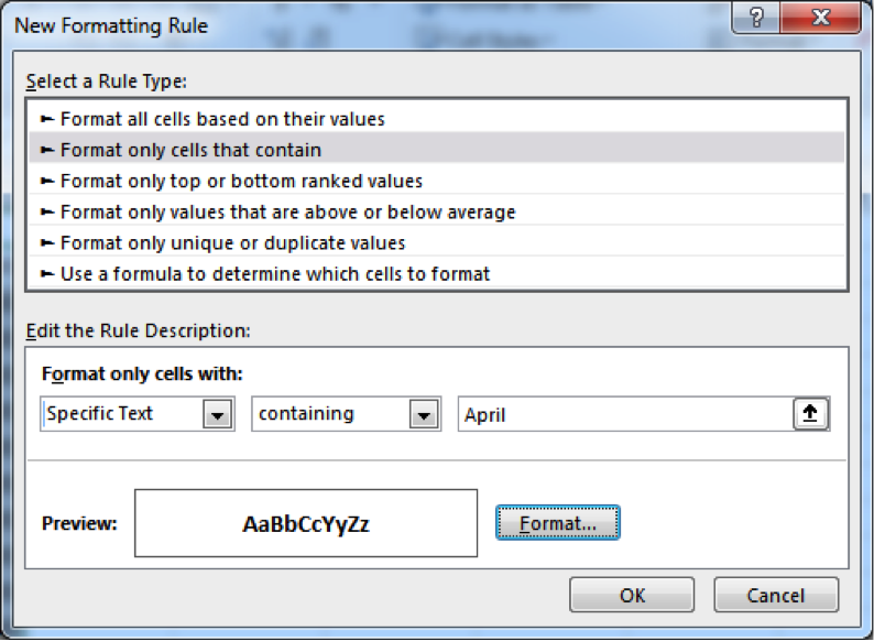
One important tool to keep in mind is the ability to enter your own rules. This can include applying formatting to specific date ranges, to specific text (like names), or even cells that are blank. In this case, you also set the format, so instead of highlighting cells you can choose to strikethrough text or change the font, change the size, or bold the text.
Practice Question
Practice Question
Candela Citations
- Formatting. Authored by: Shelli Carter. Provided by: Lumen Learning. License: CC BY: Attribution
