We have previously learned about linear equations and their line graphs.  We saw how to find the slope of a line given two points.  We also learned some ways to find the equations for a line graph.  We will now consider linear functions and their graphs. We previously learned about linear equations written in slope-intercept form, which is the form [latex]y=mx+b[/latex] where [latex]m[/latex] is the rate of change or slope and [latex]b[/latex] is the y-intercept.

The slope-intercept form is also a well-known form for writing linear functions, where [latex]f(x)[/latex] is the output value, or dependant variable, [latex]x[/latex] is the input value, or independant variable, [latex]m[/latex] is the rate of change or slope, and [latex]b[/latex] is the initial value of the dependant variable, that is [latex]b=f(0)[/latex].

[latex]\begin{array}{cc}\text{Equation form}\hfill & y=mx+b\hfill \\ \text{Function notation}\hfill & f\left(x\right)=mx+b\hfill \end{array}[/latex]

We previously learned how to calculate the slope given input and output values. Given two values for the input, [latex]{x}_{1}[/latex] and [latex]{x}_{2}[/latex], and two corresponding values for the output, [latex]{y}_{1}[/latex] and [latex]{y}_{2}[/latex] —which can be represented by a set of points, [latex]\left({x}_{1}\text{, }{y}_{1}\right)[/latex] and [latex]\left({x}_{2}\text{, }{y}_{2}\right)[/latex]—we can calculate the slope [latex]m[/latex], as follows

[latex]m=\dfrac{\text{change in output (rise)}}{\text{change in input (run)}}=\dfrac{\Delta y}{\Delta x}=\dfrac{{y}_{2}-{y}_{1}}{{x}_{2}-{x}_{1}}[/latex]

where [latex]\Delta y[/latex] is the vertical displacement and [latex]\Delta x[/latex] is the horizontal displacement.

In function notation, the corresponding values for the outputs [latex]{y}_{1}[/latex] and [latex]{y}_{2}[/latex] for the function [latex]f[/latex] are [latex]{y}_{1}=f\left({x}_{1}\right)[/latex] and [latex]{y}_{2}=f\left({x}_{2}\right)[/latex], so when using function notation we equivalently write

[latex]m=\dfrac{f\left({x}_{2}\right)-f\left({x}_{1}\right)}{{x}_{2}-{x}_{1}}[/latex]

The slope of a function is calculated by the change in [latex]y[/latex] divided by the change in [latex]x[/latex]. It does not matter which coordinate is used as the [latex]\left({x}_{2,\text{ }}f({x}_{2}\right)[/latex] and which is the [latex]\left({x}_{1},\text{ }f({x}_{1}\right))[/latex], as long as each calculation is started with the elements from the same coordinate pair.

[latex]m=\dfrac{f\left({x}_{2}\right)-f\left({x}_{1}\right)}{{x}_{2}-{x}_{1}}=\dfrac{f\left({x}_{1}\right)-f\left({x}_{2}\right)}{{x}_{1}-{x}_{2}}[/latex]

The slope provides us with important information about the graph of a linear function.  The greater the absolute value of the slope, the steeper the line is.  When the slope of a linear function is positive, the line is moving in an uphill direction from left to right across the coordinate axes. This is also called an increasing linear function. Likewise, a decreasing linear function is one whose slope is negative. The graph of a decreasing linear function is a line moving in a downhill direction from left to right across the coordinate axes.

In mathematical terms,

For a linear function [latex]f(x)=mx+b[/latex], if [latex]m>0[/latex], then [latex]f(x)[/latex] is an increasing function.

For a linear function [latex]f(x)=mx+b[/latex], if [latex]m<0[/latex], then [latex]f(x)[/latex] is a decreasing function.

For a linear function [latex]f(x)=mx+b[/latex], if [latex]m=0[/latex], then [latex]f(x)[/latex] is a constant function. Sometimes we say this is neither increasing nor decreasing.

In the following example, we will first find the slope of a linear function through two points then determine whether the line is increasing, decreasing, or neither.

In the following video we show examples of how to find the slope of a line passing through two points and then determine whether the line is increasing, decreasing or neither.

Vertical and Horizontal Lines

Vertical and horizontal lines are two special cases of linear equations.  Recall that the equation of a vertical line is given as

[latex]x=c[/latex]

where c is a constant. Regardless of the y-value of any point on the line, the x-coordinate of the point will be c.

Consider a line containing the following points: [latex]\left(-3,-5\right),\left(-3,1\right),\left(-3,3\right)[/latex], and [latex]\left(-3,5\right)[/latex].  First, we will try to find the slope.

[latex]m=\dfrac{5 - 3}{-3-\left(-3\right)}=\dfrac{2}{0}[/latex]

Zero in the denominator means that the slope is undefined.  As a result, it is impossible to write the vertical line as an equation in the form [latex]y=mx+b[/latex].

Also, recall that a function must have exactly one output for every input.  As a result, a vertical line is NOT a function. These points do not define a function because for our input, [latex]x=-3[/latex], we have an infinite number of outputs!

Although these points cannot be defined as a function, we can nevertheless plot the points.  You can see the line in the graph below. Notice that all of the x-coordinates are the same and we find a vertical line through [latex]x=-3[/latex].

The equation of a horizontal line is given as

[latex]y=c[/latex]

where c is a constant. The slope of a horizontal line is zero, and for any x-value of a point on the line, the corresponding y-coordinate will be c.

Suppose we want to find the equation of a line that contains the following set of points: [latex]\left(-2,-2\right),\left(0,-2\right),\left(3,-2\right)[/latex], and [latex]\left(5,-2\right)[/latex]. We can use point-slope form. First, we find the slope using any two points on the line.

[latex]\begin{array}{l}m & =\dfrac{-2-\left(-2\right)}{0-\left(-2\right)}\hfill \\ & =\dfrac{0}{2}\hfill \\ & =0\hfill \end{array}[/latex]

The graph is a horizontal line through [latex]y=-2[/latex]. Notice that all of the y-coordinates are the same.

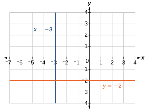
The line [latex]x=−3[/latex] is a vertical line. The line [latex]y=−2[/latex] is a horizontal line.

While we learned above that a vertical line is not a function, a horizontal line does define a function.  Recall that for a function, every input must have exactly one output.  In our example, for every input of x, the output is [latex]y=-2[/latex].  The fact that the output is always the same for every input is okay!  Notice that our horizontal line shown in the graph above passes the vertical line test because any vertical line drawn on the coordinate system will pass through the line [latex]y=-2[/latex] exactly once.

The function for our horizontal line is defined as [latex]f(x)=-2[/latex].

Contribute!

Improve this pageLearn More