Learning Outcomes
- Explain correlational research
- Describe the value of experimental research
Correlational Research
When scientists passively observe and measure phenomena it is called correlational research. Here, researchers do not intervene and change behavior, as they do in experiments. In correlational research, the goal is to identify patterns of relationships, but not cause and effect. Importantly, with correlational research, you can examine only two variables at a time, no more and no less.
So, what if you wanted to test whether spending money on others is related to happiness, but you don’t have $20 to give to each participant in order to have them spend it for your experiment? You could use a correlational design—which is exactly what Professor Elizabeth Dunn (2008) at the University of British Columbia did when she conducted research on spending and happiness. She asked people how much of their income they spent on others or donated to charity, and later she asked them how happy they were. Do you think these two variables were related? Yes, they were! The more money people reported spending on others, the happier they were.
Understanding Correlation
To find out how well two variables correlate, you can plot the relationship between the two scores on what is known as a scatterplot. In the scatterplot, each dot represents a data point. (In this case it’s individuals, but it could be some other unit.) Importantly, each dot provides us with two pieces of information—in this case, information about how good the person rated the past month (x-axis) and how happy the person felt in the past month (y-axis). Which variable is plotted on which axis does not matter.
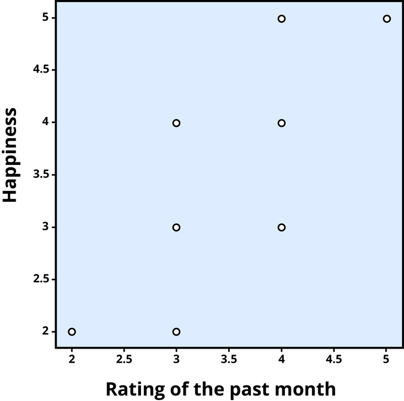
Figure 1. Scatterplot of the association between happiness and ratings of the past month, a positive correlation (r = .81). Each dot represents an individual.
The association between two variables can be summarized statistically using the correlation coefficient (abbreviated as r). A correlation coefficient provides information about the direction and strength of the association between two variables. For the example above, the direction of the association is positive. This means that people who perceived the past month as being good reported feeling more happy, whereas people who perceived the month as being bad reported feeling less happy.
With a positive correlation, the two variables go up or down together. In a scatterplot, the dots form a pattern that extends from the bottom left to the upper right (just as they do in Figure 1). The r value for a positive correlation is indicated by a positive number (although, the positive sign is usually omitted). Here, the r value is .81.
A negative correlation is one in which the two variables move in opposite directions. That is, as one variable goes up, the other goes down. Figure 2 shows the association between the average height of males in a country (y-axis) and the pathogen prevalence (or commonness of disease; x-axis) of that country. In this scatterplot, each dot represents a country. Notice how the dots extend from the top left to the bottom right. What does this mean in real-world terms? It means that people are shorter in parts of the world where there is more disease. The r value for a negative correlation is indicated by a negative number—that is, it has a minus (–) sign in front of it. Here, it is –.83.
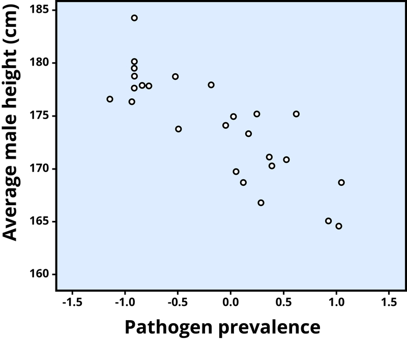
Figure 2. Scatterplot showing the association between average male height and pathogen prevalence, a negative correlation (r = –.83). Each dot represents a country (Chiao, 2009).
The strength of a correlation has to do with how well the two variables align. Recall that in Professor Dunn’s correlational study, spending on others positively correlated with happiness; the more money people reported spending on others, the happier they reported to be. At this point you may be thinking to yourself, I know a very generous person who gave away lots of money to other people but is miserable! Or maybe you know of a very stingy person who is happy as can be. Yes, there might be exceptions. If an association has many exceptions, it is considered a weak correlation. If an association has few or no exceptions, it is considered a strong correlation. A strong correlation is one in which the two variables always, or almost always, go together. In the example of happiness and how good the month has been, the association is strong. The stronger a correlation is, the tighter the dots in the scatterplot will be arranged along a sloped line.
The r value of a strong correlation will have a high absolute value (a perfect correlation has an absolute value of the whole number one, or 1.00). In other words, you disregard whether there is a negative sign in front of the r value, and just consider the size of the numerical value itself. If the absolute value is large, it is a strong correlation. A weak correlation is one in which the two variables correspond some of the time, but not most of the time. Figure 3 shows the relation between valuing happiness and grade point average (GPA). People who valued happiness more tended to earn slightly lower grades, but there were lots of exceptions to this. The r value for a weak correlation will have a low absolute value. If two variables are so weakly related as to be unrelated, we say they are uncorrelated, and the r value will be zero or very close to zero. In the previous example, is the correlation between height and pathogen prevalence strong? Compared to Figure 3, the dots in Figure 2 are tighter and less dispersed. The absolute value of –.83 is large (closer to one than to zero). Therefore, it is a strong negative correlation.
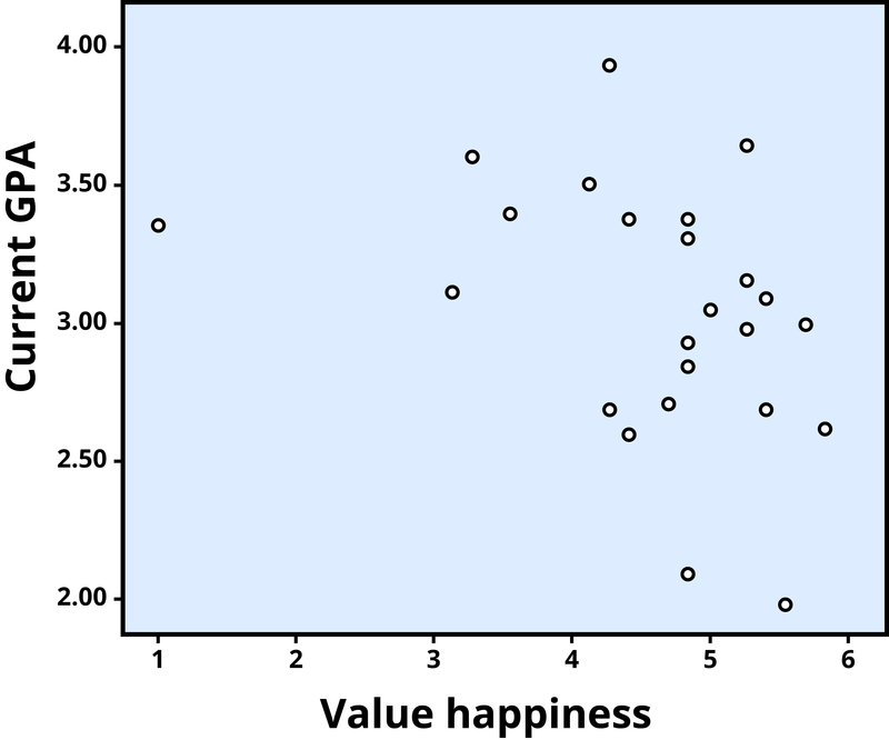
Figure 3. Scatterplot showing the association between valuing happiness and GPA, a weak negative correlation (r = –.32). Each dot represents an individual.
Problems with correlation
If generosity and happiness are positively correlated, should we conclude that being generous causes happiness? Similarly, if height and pathogen prevalence are negatively correlated, should we conclude that disease causes shortness? From a correlation alone, we can’t be certain. For example, in the first case, it may be that happiness causes generosity, or that generosity causes happiness. Or, a third variable might cause both happiness and generosity, creating the illusion of a direct link between the two. For example, wealth could be the third variable that causes both greater happiness and greater generosity. This is why correlation does not mean causation—an often repeated phrase among psychologists.
watch it
In this video, University of Pennsylvania psychologist and bestselling author, Angela Duckworth describes the correlational research that informed her understanding of grit.
link to learning
Click through this interactive presentation to examine actual research studies.
Try It
Experimental Research
Experiments are designed to test hypotheses (or specific statements about the relationship between variables) in a controlled setting in efforts to explain how certain factors or events produce outcomes. A variable is anything that changes in value. Concepts are operationalized or transformed into variables in research which means that the researcher must specify exactly what is going to be measured in the study. For example, if we are interested in studying marital satisfaction, we have to specify what marital satisfaction really means or what we are going to use as an indicator of marital satisfaction. What is something measurable that would indicate some level of marital satisfaction? Would it be the amount of time couples spend together each day? Or eye contact during a discussion about money? Or maybe a subject’s score on a marital satisfaction scale? Each of these is measurable but these may not be equally valid or accurate indicators of marital satisfaction. What do you think? These are the kinds of considerations researchers must make when working through the design.
The experimental method is the only research method that can measure cause and effect relationships between variables. Three conditions must be met in order to establish cause and effect. Experimental designs are useful in meeting these conditions:
- The independent and dependent variables must be related. In other words, when one is altered, the other changes in response. The independent variable is something altered or introduced by the researcher; sometimes thought of as the treatment or intervention. The dependent variable is the outcome or the factor affected by the introduction of the independent variable; the dependent variable depends on the independent variable. For example, if we are looking at the impact of exercise on stress levels, the independent variable would be exercise; the dependent variable would be stress.
- The cause must come before the effect. Experiments measure subjects on the dependent variable before exposing them to the independent variable (establishing a baseline). So we would measure the subjects’ level of stress before introducing exercise and then again after the exercise to see if there has been a change in stress levels. (Observational and survey research does not always allow us to look at the timing of these events which makes understanding causality problematic with these methods.)
- The cause must be isolated. The researcher must ensure that no outside, perhaps unknown variables, are actually causing the effect we see. The experimental design helps make this possible. In an experiment, we would make sure that our subjects’ diets were held constant throughout the exercise program. Otherwise, the diet might really be creating a change in stress level rather than exercise.
A basic experimental design involves beginning with a sample (or subset of a population) and randomly assigning subjects to one of two groups: the experimental group or the control group. Ideally, to prevent bias, the participants would be blind to their condition (not aware of which group they are in) and the researchers would also be blind to each participant’s condition (referred to as “double blind“). The experimental group is the group that is going to be exposed to an independent variable or condition the researcher is introducing as a potential cause of an event. The control group is going to be used for comparison and is going to have the same experience as the experimental group but will not be exposed to the independent variable. This helps address the placebo effect, which is that a group may expect changes to happen just by participating. After exposing the experimental group to the independent variable, the two groups are measured again to see if a change has occurred. If so, we are in a better position to suggest that the independent variable caused the change in the dependent variable. The basic experimental model looks like this:
| Sample is randomly assigned to one of the groups below: | Measure DV | Introduce IV | Measure DV |
|---|---|---|---|
| Experimental Group | X | X | X |
| Control Group | X | – | X |
The major advantage of the experimental design is that of helping to establish cause and effect relationships. A disadvantage of this design is the difficulty of translating much of what concerns us about human behavior into a laboratory setting.
Link to Learning
Have you ever wondered why people make decisions that seem to be in opposition to their longterm best interest? In Eldar Shafir’s TED Talk Living Under Scarcity, Shafir describes a series of experiments that shed light on how scarcity (real or perceived) affects our decisions.
Try It
Glossary
- control group:
- a comparison group that is equivalent to the experimental group, but is not given the independent variable
- correlation:
- the relationship between two or more variables; when two variables are correlated, one variable changes as the other does
- correlation coefficient:
- number from -1 to +1, indicating the strength and direction of the relationship between variables, and usually represented by r
- correlational research:
- research design with the goal of identifying patterns of relationships, but not cause and effect
- dependent variable:
- the outcome or variable that is supposedly affected by the independent variable
- double-blind:
- a research design in which neither the participants nor the researchers know whether an individual is assigned to the experimental group or the control group
- experimental group:
- the group of participants in an experiment who receive the independent variable
- experiments:
- designed to test hypotheses in a controlled setting in efforts to explain how certain factors or events produce outcomes; the only research method that measures cause and effect relationships between variables
- hypotheses:
- specific statements or predictions about the relationship between variables
- independent variable:
- something that is manipulated or introduced by the researcher to the experimental group; treatment or intervention
- negative correlation:
- two variables change in different directions, with one becoming larger as the other becomes smaller; a negative correlation is not the same thing as no correlation
- operationalized:
- concepts transformed into variables that can be measured in research
- positive correlation:
- two variables change in the same direction, both becoming either larger or smaller
- scatterplot:
- a plot or mathematical diagram consisting of data points that represent two variables
- variables:
- factors that change in value
Candela Citations
- Modification, adaptation, and original content. Provided by: Lumen Learning. License: CC BY-NC-SA: Attribution-NonCommercial-ShareAlike
- Psyc 200 Lifespan Psychology. Authored by: Laura Overstreet. Located at: http://opencourselibrary.org/econ-201/. License: CC BY: Attribution
- Research Designs. Authored by: Christie Napa Scollon. Provided by: Singapore Management University. Project: The Noba Project. License: CC BY-NC-SA: Attribution-NonCommercial-ShareAlike
- Vocabulary and review about correlational research. Provided by: Lumen Learning. Located at: https://courses.lumenlearning.com/waymaker-psychology/wp-admin/post.php?post=1848&action=edit. License: CC BY: Attribution
- Grit: The power of passion and perseverance. Authored by: Angela Lee Duckworth. Provided by: TED. Located at: https://www.ted.com/talks/angela_lee_duckworth_grit_the_power_of_passion_and_perseverance. License: CC BY-NC-ND: Attribution-NonCommercial-NoDerivatives