Learning Objectives
- Explain the investment, government spending, and net export functions
- Explain how the aggregate expenditure curve is constructed from the consumption, investment, government spending and net export functions
Aggregate Expenditure = C + I + G + (X – M).
Now let’s turn our attention to the other components in order to build a function for the total aggregate expenditures.
Aggregate Expenditure: Investment as a Function of National Income
Just as a consumption function shows the relationship between real GDP (or national income) and consumption levels, the investment function shows the relationship between real GDP and investment levels. When businesses make decisions about whether to build a new factory or to place an order for new computer equipment, their decision is forward-looking, based on expected rates of return, and the interest rate at which they can borrow for the investment expenditure. Investment decisions do not depend primarily on the level of GDP in the current year. Thus, the investment function can be drawn as a horizontal line, at a fixed level of expenditure. The slope of the investment function is zero, indicating no relationship between GDP and investment. Figure 1 shows an investment function where the level of investment is, for the sake of concreteness, set at the specific level of 500.
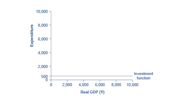
Figure 1. The Investment Function. The investment function is drawn as a horizontal line because investment is based on interest rates and expectations about the future, and so it does not change with the level of current national income. In this example, investment expenditures are at a level of 500. However, changes in factors like technological opportunities, expectations about near-term economic growth, and interest rates would all cause the investment function to shift up or down.
The appearance of the investment function as a horizontal line does not mean that the level of investment never changes. It means only that in the context of this two-dimensional diagram, the level of investment on the vertical aggregate expenditure axis does not vary with changes in the current level of GDP on the horizontal axis. However, all the other factors that influence investment—new technological opportunities, expectations about near-term economic growth, interest rates, the price of key inputs, and tax incentives for investment—can cause the horizontal investment function to shift up or down.
Aggregate Expenditure: Government Spending and Taxes as a Function of National Income
Federal, state and local governments determine the level of government spending through the budget process. In the Keynesian cross diagram, government spending appears as a horizontal line, as in Figure 2, where government spending is set at a level of 1,300 regardless of the level of GDP. As in the case of investment spending, this horizontal line does not mean that government spending is unchanging, only that it is independent of GDP.
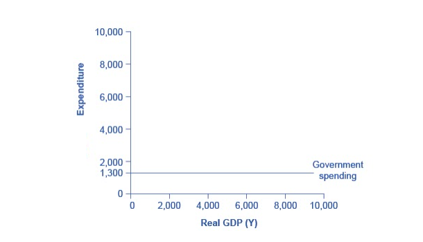
Figure 2. The Government Spending Function. The level of government spending is determined by political factors, not by the level of real GDP in a given year. Thus, government spending is drawn as a horizontal line. In this example, government spending is at a level of 1,300. Congressional decisions to increase government spending will cause this horizontal line to shift up, while decisions to reduce spending would cause it to shift down.
The situation of taxes is different because taxes typically rise or fall with the volume of economic activity. For example, income taxes are based on the level of income earned and sales taxes are based on the amount of sales made, and both income and sales tend to be higher when the economy is growing and lower when the economy is in a recession. For the purposes of constructing the basic Keynesian cross diagram, tax revenues can be viewed as the product of the average tax rate (economy-wide) times the national income (or GDP). In the United States, for example, taking federal, state, and local taxes together, government typically collects about 30–35% of national income as taxes.
Table 2 revises the earlier table on the consumption function so that it takes taxes into account. The first column shows national income. The second column calculates taxes, which in this example are set at a rate of 30%, or 0.3. The third column shows after-tax income; that is, total income minus taxes. The fourth column then calculates consumption in the same manner as before: multiply after-tax income by 0.8, representing the marginal propensity to consume, and then add $600, for the amount that would be consumed even if income was zero. When taxes are included, the marginal propensity to consume is reduced by the amount of the tax rate, so each additional dollar of income results in a smaller increase in consumption than before taxes. For this reason, the consumption function, with taxes included, is flatter than the consumption function without taxes, as Figure 3 shows.
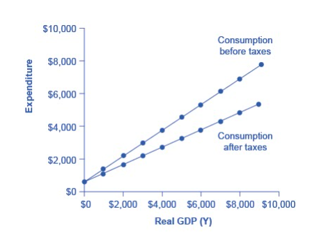
Figure 3. The Consumption Function Before and After Taxes. The upper line repeats the consumption function from previously. The lower line shows the consumption function if taxes must first be paid on income, and then consumption is based on after-tax income.
| Income | Taxes | After-Tax Income | Consumption | Savings |
|---|---|---|---|---|
| $0 | $0 | $0 | $600 | –$600 |
| $1,000 | $300 | $700 | $1,160 | –$460 |
| $2,000 | $600 | $1,400 | $1,720 | –$320 |
| $3,000 | $900 | $2,100 | $2,280 | –$180 |
| $4,000 | $1,200 | $2,800 | $2,840 | –$40 |
| $5,000 | $1,500 | $3,500 | $3,400 | $100 |
| $6,000 | $1,800 | $4,200 | $3,960 | $240 |
| $7,000 | $2,100 | $4,900 | $4,520 | $380 |
| $8,000 | $2,400 | $5,600 | $5,080 | $520 |
| $9,000 | $2,700 | $6,300 | $5,640 | $660 |
Try It
Aggregate Expenditure: Net Exports as a Function of National Income
Aggregate Expenditure means spending on domestically produced goods and services. There are two additional things we need to consider: exports and imports. This is especially true in the increasingly global world of the 21st Century. Exports are purchases by foreigners of domestically produced goods and services, which means exports contribute to aggregate expenditure. Imports are purchases of foreign goods and services by domestic residents, which means that spending on imports takes away from spending on domestic goods and services. Let’s consider how imports and exports can be graphed as a function of national income (or real GDP).
The demand for imported goods and services is a subset of the demand for goods and services generally. We’ve established that consumption expenditure increases with national income; thus in a macroeconomic context, the same thing is true of imports—the purchase of imports increases with national income. The demand by foreigners for our exports depends on their national income, but it is independent of our domestic national income. We can draw these two relationships as the export and import functions, shown below in Figures 4a and 4b.
The export function, which shows how exports change with the level of a country’s own real GDP, is drawn as a horizontal line, as in the example in Figure 4(a) where exports are drawn at a level of $840. Again, as in the case of investment spending and government spending, drawing the export function as horizontal does not imply that exports never change. It just means that they do not change because of what is on the horizontal axis—that is, a country’s national income (or GDP)—and instead are shaped by the level of aggregate demand in other countries. More demand for exports from other countries would cause the export function to shift up; less demand for exports from other countries would cause it to shift down.
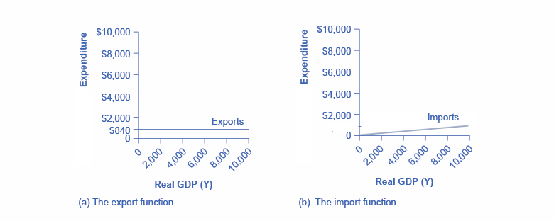
Figure 4. The Export and Import Functions. (a) The export function is drawn as a horizontal line because exports are determined by the buying power of other countries and thus do not change with the size of the domestic economy. In this example, exports are set at 840. However, exports can shift up or down, depending on buying patterns in other countries. (b) The import function is drawn as an upward-sloping line because expenditures on imported products increase with income. In this example, the marginal propensity to import is 0.1, so imports are calculated by multiplying the level of income by +0.1.
The import function, as explained above, is an upward-sloping line, showing that as national income rises so do import expenditures. The slope is given by the marginal propensity to import (MPI), which is the percentage change in spending on imports when national income changes.
In Figure 4(b), the marginal propensity to import is 0.1. Thus, if real GDP is $5,000, imports are $500; if real GDP is $6,000, imports are $600, and so on. A change in the marginal propensity to import, perhaps as a result of changes in preferences, would alter the slope of the import function.
Let’s put these ideas together. The balance of international trade in a country is called Net Exports in this model. Net Exports is defined as the value of a country’s exports minus the value of its imports. Thus, a trade surplus means a country’s exports are greater than its imports and a trade deficit means the country’s imports are greater than its exports. A trade surplus is a net addition to a country’s aggregate expenditure and a trade deficit is a net subtraction.
When imports are subtracted from exports, we get a downward-sloping line with a slope equal to -MPI. In other words, the higher the national income, the more imports a country purchases and the less it spends on domestic goods and services. Thus, net exports decrease with national income (or real GDP).
Putting It Together: The Aggregate Expenditure Function
The final step in deriving the aggregate expenditure function, which shows the total expenditures in the economy for each level of real GDP, is to sum the parts, which is shown in Table 3.
| Real GDP | Consumption (C) | Investment (I) | Government Spending (G) | Exports (X) | Imports (M) | Net Exports (X-M) | Aggregate Expenditure (AE) |
|---|---|---|---|---|---|---|---|
| $0 | $600 | $500 | $1,300 | $840 | $0 | $840 | $3,240 |
| $1,000 | $1,160 | $500 | $1,300 | $840 | $100 | $740 | $3,700 |
| $2,000 | $1,720 | $500 | $1,300 | $840 | $200 | $640 | $4,160 |
| $3,000 | $2,280 | $500 | $1,300 | $840 | $300 | $540 | $4,620 |
| $4,000 | $2,840 | $500 | $1,300 | $840 | $400 | $440 | $5,080 |
| $5,000 | $3,400 | $500 | $1,300 | $840 | $500 | $340 | $5,540 |
| $6,000 | $3,960 | $500 | $1,300 | $840 | $600 | $240 | $6,000 |
| $7,000 | $4,520 | $500 | $1,300 | $840 | $700 | $140 | $6,460 |
| $8,000 | $5,080 | $500 | $1,300 | $840 | $800 | $40 | $6,920 |
| $9,000 | $5,640 | $500 | $1,300 | $840 | $900 | -$60 | $7,380 |
Each of the columns in Table 3 comes from the previous tables and figures. For example the second column, consumption, comes from Table 2, and the seventh column, net exports, is computed from the numbers in Figure 4. Taking national income (or Real GDP) from column 1 and aggregate expenditure from column 6, we can graph the aggregate expenditure function.
Graphically, the aggregate expenditure function is formed by adding together (or stacking on top of each other) the consumption function (after taxes), the investment function, the government spending function, and the net export function. In its most basic form, the graph of aggregate expenditures looks like the graph shown in Figure 5.
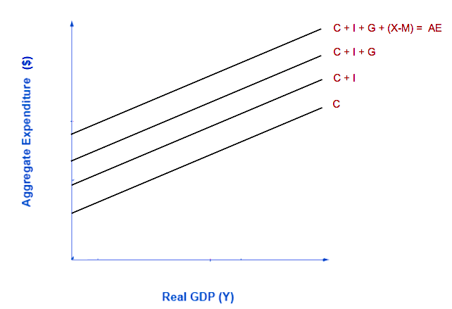
Figure 5. Graphing Aggregate Expenditure. The aggregate expenditure is the vertical sum of C + I + G + (X-M).
Try It
Try It
These questions allow you to get as much practice as you need, as you can click the link at the top of the first question (“Try another version of these questions”) to get a new set of questions. Practice until you feel comfortable doing the questions.
Glossary
- Aggregate Expenditure Function:
- graphical relationship between national income as a function of aggregate expenditure, which is defined as consumption plus investment plus government spending plus net exports
- Aggregate Expenditure Schedule:
- aggregate expenditure function expressed as a table
- Autonomous Expenditures:
- the sum of the components of aggregate expenditure that do not vary with national income; these include autonomous consumption, investment, government, and export expenditures
- Consumption Function:
- graphical relationship between national income and consumption expenditure; algebraically: C = a + MPC*Y, where a is autonomous consumption (the amount of consumption expenditure when Y = 0), MPC is the marginal propensity to consume, and Y is national income
- Government Spending Function:
- horizontal line showing the relationship between national income and government spending
- Investment Expenditure Function:
- horizontal line showing the relationship between national income and investment expenditure
- Marginal Propensity to Consume:
- fraction of any change in income which is spent; algebraically MPC =ΔC /ΔY
- Marginal Propensity to Import:
- fraction of any change in income which is spent on imports; algebraically MPI =ΔM /ΔY
- Marginal Propensity to Save:
- fraction of any change in income which is saved; algebraically MPS = ΔS /ΔY
- Net Export Function:
- graphical relationship between national income and net exports (export expenditures minus import expenditures)
Candela Citations
- Modification, adaptation, and original content. Provided by: Lumen Learning. License: CC BY: Attribution
- The Expenditure-Output Model. Authored by: OpenStax College. Located at: https://cnx.org/contents/QGHIMgmO@11.12:LJYhl4AE@11/The-Expenditure-Output-Model. License: CC BY: Attribution. License Terms: Download for free at http://cnx.org/contents/4061c832-098e-4b3c-a1d9-7eb593a2cb31@11.11
