Learning Objectives
- Explain and graph the consumption function
- Explain what would cause the consumption function to grow steeper or flatter, or to shift up or down
Aggregate Expenditure: Consumption as a Function of National Income
Keynes observed that consumption expenditure depends primarily on personal disposable income, i.e. one’s take home pay. Let’s examine this relationship in more detail. People can do two things with their income: they can consume it or they can save it. (For the moment, let’s ignore the need to pay taxes with some of it). Each person who receives a raise in income faces this choice. Let’s define the marginal propensity to consume (MPC) as the share (or percentage) of the additional income a person decides to consume (or spend). Similarly, the marginal propensity to save (MPS) is the share of the additional income the person decides to save. Since the only options are to consume or save income, it must always hold true that:
For example, if the marginal propensity to consume out of the marginal amount of income earned is 0.9, then the marginal propensity to save is 0.1.
With this relationship in mind, consider the relationship among income, consumption, and savings shown in Table 1.
| Income | Consumption | Savings |
|---|---|---|
| $0 | $600 | –$600 |
| $1,000 | $1,400 | –$400 |
| $2,000 | $2,200 | –$200 |
| $3,000 | $3,000 | $0 |
| $4,000 | $3,800 | $200 |
| $5,000 | $4,600 | $400 |
| $6,000 | $5,400 | $600 |
| $7,000 | $6,200 | $800 |
| $8,000 | $7,000 | $1,000 |
| $9,000 | $7,800 | $1,200 |
In Table 1, for each increase in income of $1000, consumption increases by $800. Thus, the marginal propensity to consumer (MPC) is 0.80. Any additional income which isn’t spent is saved, so for each increase in income of $1000, saving increases by $200. The MPS is 0.20.
Try It
The pattern of consumption shown in Table 1 is plotted in Figure 1. The relationship between income and consumption, whether in tabular or graphical form is called the consumption function. Both the table and figure illustrate a typical consumption function. There are a couple of features to observe. First, consumption expenditure increases as income does. For every increase in income, consumption increases by the MPC times that increase in income. Thus, the slope of the consumption function is the MPC. Second, at low levels of income, consumption is greater than income. Even if income were zero, people would have to consume something. We call the level of consumption when income is zero autonomous consumption since it shows the amount of consumption independent of income. In this example, consumption would be $600 even if income were zero. Thus, to calculate consumption at any level of income, multiply the income level by 0.8, for the marginal propensity to consume, and add $600, for the amount that would be consumed even if income was zero.
C = 600 + 0.8*Y
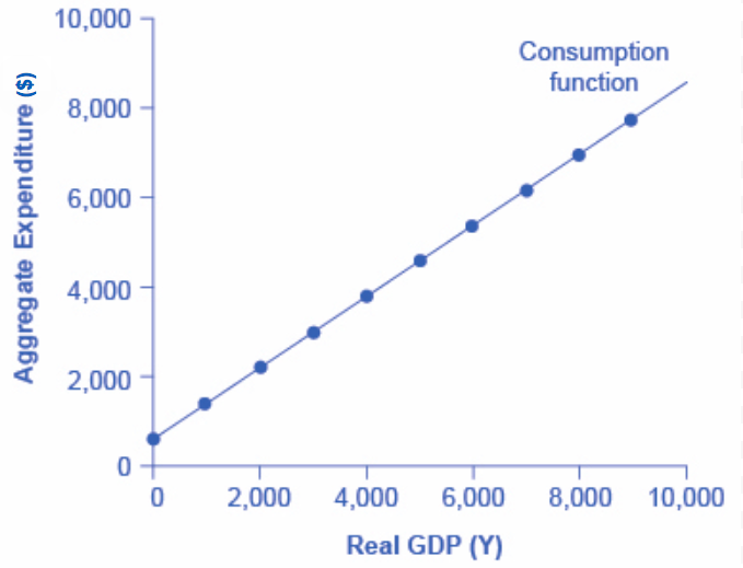
Figure 1. The Consumption Function. In the expenditure-output model, how does consumption increase with the level of national income? Output on the horizontal axis is conceptually the same as national income, since the value of all final output that is produced and sold must be income to someone, somewhere in the economy. At a national income level of zero, $600 is consumed. Then, each time income rises by $1,000, consumption rises by $800, because in this example, the marginal propensity to consume is 0.8.
A change in the marginal propensity to consume will change the slope of the consumption function. An increase in the MPC steepens the consumption function; a decrease in the MPC flattens it.
Try It
A number of factors other than income can also cause the entire consumption function to shift. These factors were summarized in the earlier discussion of consumption. For example, changes in consumer expectations about the future, or changes in household wealth would cause the consumption function to shift up or down to a new consumption function that is parallel to the original one.
Watch It
Watch the selected three-minute clip from this video to take another look at the consumption function and the marginal propensity to consume. Note that his graph is a rough sketch and not drawn entirely to scale.
You can view the transcript for “Consumption Function” here (opens in new window).
Watch this next video for more practice in graphing the consumption function. Then take it a step further to analyze what kind of impact an increase in income will have on consumer spending.
You can view the transcript for “Consumption function” here (opens in new window).
Try It
These questions allow you to get as much practice as you need, as you can click the link at the top of the first question (“Try another version of these questions”) to get a new set of questions. Practice until you feel comfortable doing the questions.
Try It
These questions allow you to get as much practice as you need, as you can click the link at the top of the first question (“Try another version of these questions”) to get a new set of questions. Practice until you feel comfortable doing the questions.
Glossary
- autonomous consumption:
- The amount consumers spend if their income was zero; i.e. consumer spending which is caused by something other than income, for example, borrowing
- consumption function:
- graphical relationship between national income and consumption expenditure; algebraically: C = a + MPC*Y, where a is autonomous consumption (the amount of consumption expenditure when Y = 0), MPC is the marginal propensity to consume, and Y is national income
- marginal propensity to consume:
- fraction of any change in income which is spent; algebraically MPC = ΔC/ΔY
- marginal propensity to save:
- fraction of any change in income which is saved; algebraically MPS = ΔS/ΔY
Candela Citations
- Modification, adaptation, and original content. Provided by: Lumen Learning. License: CC BY: Attribution
- The Expenditure-Output Model. Authored by: OpenStax College. Located at: https://cnx.org/contents/vEmOH-_p@4.29:2cZ9K6tp@3/The-Expenditure-Output-Model. License: CC BY: Attribution. License Terms: Download for free at http://cnx.org/contents/bc498e1f-efe9-43a0-8dea-d3569ad09a82@4.4
- Consumption Function. Provided by: lostmy1. Located at: https://www.youtube.com/watch?v=G5XQB7vZqvA. License: CC BY: Attribution
- Consumption Function. Authored by: Collin Weigel. Located at: https://www.youtube.com/watch?time_continue=4&v=_iuj76W76Ts. License: Other. License Terms: Standard YouTube License