Learning Outcomes
- Identify zeros of polynomial functions with even and odd multiplicity.
- Draw the graph of a polynomial function using end behavior, turning points, intercepts, and the Intermediate Value Theorem.
- Write the equation of a polynomial function given its graph.
The revenue in millions of dollars for a fictional cable company from 2006 through 2013 is shown in the table below.
| Year | 2006 | 2007 | 2008 | 2009 | 2010 | 2011 | 2012 | 2013 |
| Revenue | 52.4 | 52.8 | 51.2 | 49.5 | 48.6 | 48.6 | 48.7 | 47.1 |
The revenue can be modeled by the polynomial function
[latex]R\left(t\right)=-0.037{t}^{4}+1.414{t}^{3}-19.777{t}^{2}+118.696t - 205.332[/latex]
where R represents the revenue in millions of dollars and t represents the year, with t = 6 corresponding to 2006. Over which intervals is the revenue for the company increasing? Over which intervals is the revenue for the company decreasing? These questions, along with many others, can be answered by examining the graph of the polynomial function. We have already explored the local behavior of quadratics, a special case of polynomials. In this section we will explore the local behavior of polynomials in general.
Multiplicity and Turning Points
Graphs behave differently at various x-intercepts. Sometimes the graph will cross over the x-axis at an intercept. Other times the graph will touch the x-axis and bounce off.
Suppose, for example, we graph the function [latex]f\left(x\right)=\left(x+3\right){\left(x - 2\right)}^{2}{\left(x+1\right)}^{3}[/latex].
Notice in the figure below that the behavior of the function at each of the x-intercepts is different.
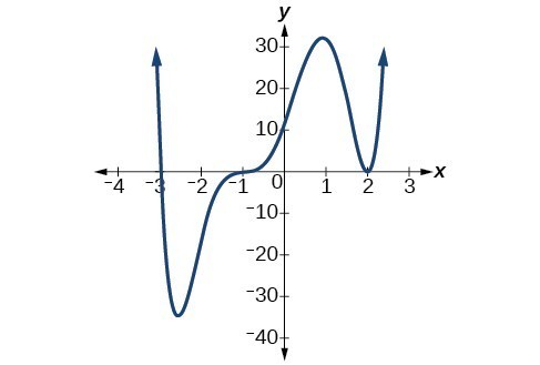
The behavior of a graph at an x-intercept can be determined by examining the multiplicity of the zero.
The x-intercept [latex]x=-3[/latex] is the solution to the equation [latex]\left(x+3\right)=0[/latex]. The graph passes directly through the x-intercept at [latex]x=-3[/latex]. The factor is linear (has a degree of 1), so the behavior near the intercept is like that of a line; it passes directly through the intercept. We call this a single zero because the zero corresponds to a single factor of the function.
The x-intercept [latex]x=2[/latex] is the repeated solution to the equation [latex]{\left(x - 2\right)}^{2}=0[/latex]. The graph touches the axis at the intercept and changes direction. The factor is quadratic (degree 2), so the behavior near the intercept is like that of a quadratic—it bounces off of the horizontal axis at the intercept.
[latex]{\left(x - 2\right)}^{2}=\left(x - 2\right)\left(x - 2\right)[/latex]
The factor is repeated, that is, the factor [latex]\left(x - 2\right)[/latex] appears twice. The number of times a given factor appears in the factored form of the equation of a polynomial is called the multiplicity. The zero associated with this factor, [latex]x=2[/latex], has multiplicity 2 because the factor [latex]\left(x - 2\right)[/latex] occurs twice.
The x-intercept [latex]x=-1[/latex] is the repeated solution of factor [latex]{\left(x+1\right)}^{3}=0[/latex]. The graph passes through the axis at the intercept but flattens out a bit first. This factor is cubic (degree 3), so the behavior near the intercept is like that of a cubic with the same S-shape near the intercept as the function [latex]f\left(x\right)={x}^{3}[/latex]. We call this a triple zero, or a zero with multiplicity 3.
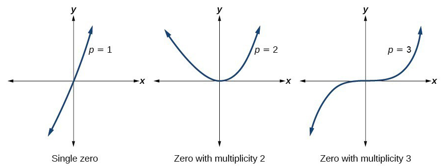
For zeros with even multiplicities, the graphs touch or are tangent to the x-axis at these x-values. For zeros with odd multiplicities, the graphs cross or intersect the x-axis at these x-values. See the graphs below for examples of graphs of polynomial functions with multiplicity 1, 2, and 3.
For higher even powers, such as 4, 6, and 8, the graph will still touch and bounce off of the x-axis, but for each increasing even power the graph will appear flatter as it approaches and leaves the x-axis.
For higher odd powers, such as 5, 7, and 9, the graph will still cross through the x-axis, but for each increasing odd power, the graph will appear flatter as it approaches and leaves the x-axis.
A General Note: Graphical Behavior of Polynomials at x-Intercepts
If a polynomial contains a factor of the form [latex]{\left(x-h\right)}^{p}[/latex], the behavior near the x-intercept h is determined by the power p. We say that [latex]x=h[/latex] is a zero of multiplicity p.
The graph of a polynomial function will touch the x-axis at zeros with even multiplicities. The graph will cross the x-axis at zeros with odd multiplicities.
The sum of the multiplicities is the degree of the polynomial function.
How To: Given a graph of a polynomial function of degree [latex]n[/latex], identify the zeros and their multiplicities.
- If the graph crosses the x-axis and appears almost linear at the intercept, it is a single zero.
- If the graph touches the x-axis and bounces off of the axis, it is a zero with even multiplicity.
- If the graph crosses the x-axis at a zero, it is a zero with odd multiplicity.
- The sum of the multiplicities is the degree n.
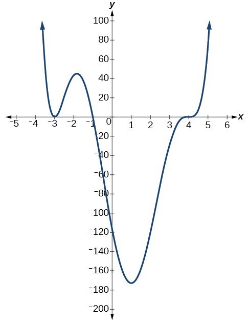
Example: Identifying Zeros and Their Multiplicities
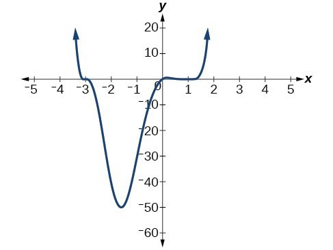
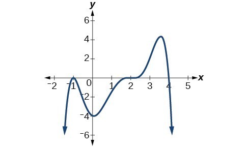
Use the graph of the function of degree 6 to identify the zeros of the function and their possible multiplicities.
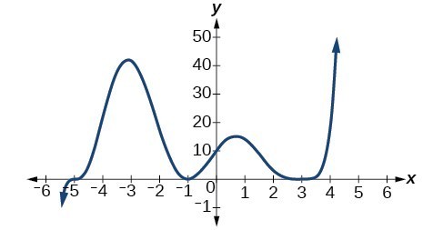
Try It
Use the graph of the function of degree 7 to identify the zeros of the function and their multiplicities.
Determining End Behavior
As we have already learned, the behavior of a graph of a polynomial function of the form
[latex]f\left(x\right)={a}_{n}{x}^{n}+{a}_{n - 1}{x}^{n - 1}+...+{a}_{1}x+{a}_{0}[/latex]
will either ultimately rise or fall as x increases without bound and will either rise or fall as x decreases without bound. This is because for very large inputs, say 100 or 1,000, the leading term dominates the size of the output. The same is true for very small inputs, say –100 or –1,000.
Recall that we call this behavior the end behavior of a function. As we pointed out when discussing quadratic equations, when the leading term of a polynomial function, [latex]{a}_{n}{x}^{n}[/latex], is an even power function, as x increases or decreases without bound, [latex]f\left(x\right)[/latex] increases without bound. When the leading term is an odd power function, as x decreases without bound, [latex]f\left(x\right)[/latex] also decreases without bound; as x increases without bound, [latex]f\left(x\right)[/latex] also increases without bound. If the leading term is negative, it will change the direction of the end behavior. The table below summarizes all four cases.
| Even Degree | Odd Degree |
|---|---|
 |
 |
 |
 |
Try It
Graphing Polynomial Functions
We can use what we have learned about multiplicities, end behavior, and turning points to sketch graphs of polynomial functions. Let us put this all together and look at the steps required to graph polynomial functions.
How To: Given a polynomial function, sketch the graph
- Find the intercepts.
- Check for symmetry. If the function is an even function, its graph is symmetric with respect to the y-axis, that is, f(–x) = f(x).
If a function is an odd function, its graph is symmetric with respect to the origin, that is, f(–x) = –f(x). - Use the multiplicities of the zeros to determine the behavior of the polynomial at the x-intercepts.
- Determine the end behavior by examining the leading term.
- Use the end behavior and the behavior at the intercepts to sketch the graph.
- Ensure that the number of turning points does not exceed one less than the degree of the polynomial.
- Optionally, use technology to check the graph.
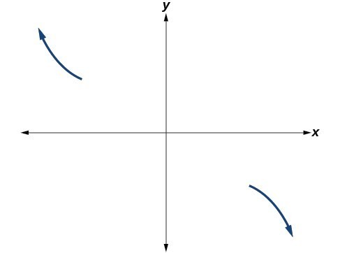
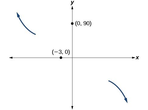
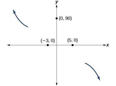
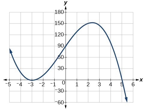
Example: Sketching the Graph of a Polynomial Function
Sketch a possible graph for [latex]f\left(x\right)=-2{\left(x+3\right)}^{2}\left(x - 5\right)[/latex].
Try It
Sketch a possible graph for [latex]f\left(x\right)=\frac{1}{4}x{\left(x - 1\right)}^{4}{\left(x+3\right)}^{3}[/latex].
The Intermediate Value Theorem
In some situations, we may know two points on a graph but not the zeros. If those two points are on opposite sides of the x-axis, we can confirm that there is a zero between them. Consider a polynomial function f whose graph is smooth and continuous. The Intermediate Value Theorem states that for two numbers a and b in the domain of f, if a < b and [latex]f\left(a\right)\ne f\left(b\right)[/latex], then the function f takes on every value between [latex]f\left(a\right)[/latex] and [latex]f\left(b\right)[/latex].
We can apply this theorem to a special case that is useful for graphing polynomial functions. If a point on the graph of a continuous function f at [latex]x=a[/latex] lies above the x-axis and another point at [latex]x=b[/latex] lies below the x-axis, there must exist a third point between [latex]x=a[/latex] and [latex]x=b[/latex] where the graph crosses the x-axis. Call this point [latex]\left(c,\text{ }f\left(c\right)\right)[/latex]. This means that we are assured there is a value c where [latex]f\left(c\right)=0[/latex].
In other words, the Intermediate Value Theorem tells us that when a polynomial function changes from a negative value to a positive value, the function must cross the x-axis. The figure below shows that there is a zero between a and b.
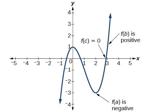
The Intermediate Value Theorem can be used to show there exists a zero.
A General Note: Intermediate Value Theorem
Let f be a polynomial function. The Intermediate Value Theorem states that if [latex]f\left(a\right)[/latex] and [latex]f\left(b\right)[/latex] have opposite signs, then there exists at least one value c between a and b for which [latex]f\left(c\right)=0[/latex].
Example: Using the Intermediate Value Theorem
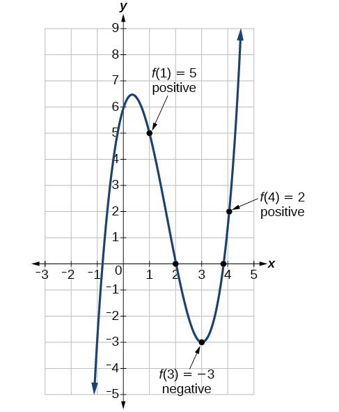
Show that the function [latex]f\left(x\right)={x}^{3}-5{x}^{2}+3x+6[/latex] has at least two real zeros between [latex]x=1[/latex] and [latex]x=4[/latex].
Try It
Show that the function [latex]f\left(x\right)=7{x}^{5}-9{x}^{4}-{x}^{2}[/latex] has at least one real zero between [latex]x=1[/latex] and [latex]x=2[/latex].
Writing Formulas for Polynomial Functions
Now that we know how to find zeros of polynomial functions, we can use them to write formulas based on graphs. Because a polynomial function written in factored form will have an x-intercept where each factor is equal to zero, we can form a function that will pass through a set of x-intercepts by introducing a corresponding set of factors.
A General Note: Factored Form of Polynomials
If a polynomial of lowest degree p has zeros at [latex]x={x}_{1},{x}_{2},\dots ,{x}_{n}[/latex], then the polynomial can be written in the factored form: [latex]f\left(x\right)=a{\left(x-{x}_{1}\right)}^{{p}_{1}}{\left(x-{x}_{2}\right)}^{{p}_{2}}\cdots {\left(x-{x}_{n}\right)}^{{p}_{n}}[/latex] where the powers [latex]{p}_{i}[/latex] on each factor can be determined by the behavior of the graph at the corresponding intercept, and the stretch factor a can be determined given a value of the function other than the x-intercept.
How To: Given a graph of a polynomial function, write a formula for the function
- Identify the x-intercepts of the graph to find the factors of the polynomial.
- Examine the behavior of the graph at the x-intercepts to determine the multiplicity of each factor.
- Find the polynomial of least degree containing all of the factors found in the previous step.
- Use any other point on the graph (the y-intercept may be easiest) to determine the stretch factor.
Example: Writing a Formula for a Polynomial Function from Its Graph
Write a formula for the polynomial function.
Try It
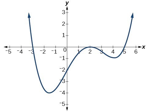
Given the graph below, write a formula for the function shown.
Local and Global Extrema
With quadratics, we were able to algebraically find the maximum or minimum value of the function by finding the vertex. For general polynomials, finding these turning points is not possible without more advanced techniques from calculus. Even then, finding where extrema occur can still be algebraically challenging. For now, we will estimate the locations of turning points using technology to generate a graph.
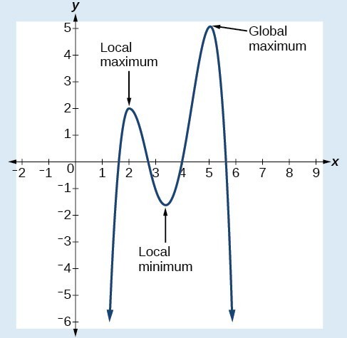
Each turning point represents a local minimum or maximum. Sometimes, a turning point is the highest or lowest point on the entire graph. In these cases, we say that the turning point is a global maximum or a global minimum. These are also referred to as the absolute maximum and absolute minimum values of the function.
A local maximum or local minimum at x = a (sometimes called the relative maximum or minimum, respectively) is the output at the highest or lowest point on the graph in an open interval around x = a. If a function has a local maximum at a, then [latex]f\left(a\right)\ge f\left(x\right)[/latex] for all x in an open interval around x = a. If a function has a local minimum at a, then [latex]f\left(a\right)\le f\left(x\right)[/latex] for all x in an open interval around x = a.
A global maximum or global minimum is the output at the highest or lowest point of the function. If a function has a global maximum at a, then [latex]f\left(a\right)\ge f\left(x\right)[/latex] for all x. If a function has a global minimum at a, then [latex]f\left(a\right)\le f\left(x\right)[/latex] for all x.
We can see the difference between local and global extrema below.
Q & A
Do all polynomial functions have a global minimum or maximum?
No. Only polynomial functions of even degree have a global minimum or maximum. For example, [latex]f\left(x\right)=x[/latex] has neither a global maximum nor a global minimum.
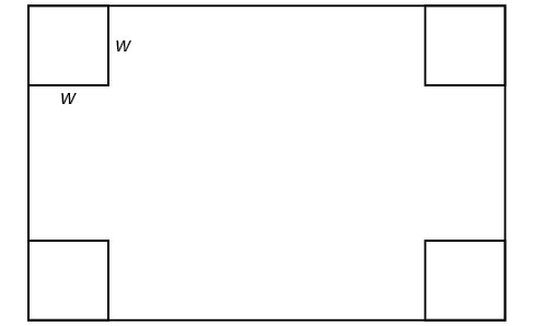
Example: Using Local Extrema to Solve Applications
An open-top box is to be constructed by cutting out squares from each corner of a 14 cm by 20 cm sheet of plastic then folding up the sides. Find the size of squares that should be cut out to maximize the volume enclosed by the box.
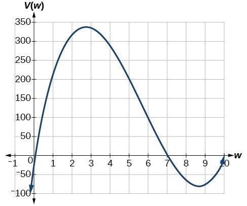
![Graph of V(w)=(20-2w)(14-2w)w where the x-axis is labeled w and the y-axis is labeled V(w) on the domain [2.4, 3].](https://s3-us-west-2.amazonaws.com/courses-images/wp-content/uploads/sites/896/2016/11/02201637/CNX_Precalc_Figure_03_04_0292.jpg)
Key Concepts
- Polynomial functions of degree 2 or more are smooth, continuous functions.
- To find the zeros of a polynomial function, if it can be factored, factor the function and set each factor equal to zero.
- Another way to find the x-intercepts of a polynomial function is to graph the function and identify the points where the graph crosses the x-axis.
- The multiplicity of a zero determines how the graph behaves at the x-intercept.
- The graph of a polynomial will cross the x-axis at a zero with odd multiplicity.
- The graph of a polynomial will touch and bounce off the x-axis at a zero with even multiplicity.
- The end behavior of a polynomial function depends on the leading term.
- The graph of a polynomial function changes direction at its turning points.
- A polynomial function of degree n has at most n – 1 turning points.
- To graph polynomial functions, find the zeros and their multiplicities, determine the end behavior, and ensure that the final graph has at most n – 1 turning points.
- Graphing a polynomial function helps to estimate local and global extremas.
- The Intermediate Value Theorem tells us that if [latex]f\left(a\right) \text{and} f\left(b\right)[/latex] have opposite signs, then there exists at least one value c between a and b for which [latex]f\left(c\right)=0[/latex].
Glossary
- global maximum
- highest turning point on a graph; [latex]f\left(a\right)[/latex] where [latex]f\left(a\right)\ge f\left(x\right)[/latex] for all x.
- global minimum
- lowest turning point on a graph; [latex]f\left(a\right)[/latex] where [latex]f\left(a\right)\le f\left(x\right)[/latex] for all x.
- Intermediate Value Theorem
- for two numbers a and b in the domain of f, if [latex]a
- multiplicity
- the number of times a given factor appears in the factored form of the equation of a polynomial; if a polynomial contains a factor of the form [latex]{\left(x-h\right)}^{p}[/latex], [latex]x=h[/latex] is a zero of multiplicity p.
Candela Citations
- Revision and Adaptation. Provided by: Lumen Learning. License: CC BY: Attribution
- Question ID 121830. Authored by: Lumen Learning. License: CC BY: Attribution. License Terms: IMathAS Community License CC-BY + GPL
- College Algebra. Authored by: Abramson, Jay et al.. Provided by: OpenStax. Located at: http://cnx.org/contents/9b08c294-057f-4201-9f48-5d6ad992740d@5.2. License: CC BY: Attribution. License Terms: Download for free at http://cnx.org/contents/9b08c294-057f-4201-9f48-5d6ad992740d@5.2
- Question ID 29470, 29478. Authored by: Caren McClure. License: CC BY: Attribution. License Terms: IMathAS Community License CC-BY + GPL