Learning Outcomes
- Identify power functions.
- Describe end behavior of power functions given its equation or graph.
- Identify polynomial functions.
- Identify the degree and leading coefficient of polynomial functions.
- Describe the end behavior of a polynomial function.
- Identify turning points of a polynomial function from its graph.
- Identify the number of turning points and intercepts of a polynomial function from its degree.
- Determine x and y-intercepts of a polynomial function given its equation in factored form.
In this section we will examine functions that are used to estimate and predict things like changes in animal and bird populations or fluctuations in financial markets.
We will also continue to learn how to analyze the behavior of functions by looking at their graphs. We will introduce and describe a new term called end behavior and show which parts of the function equation determine end behavior. We will also identify intercepts of polynomial functions.
End Behavior of Power Functions

Three birds on a cliff with the sun rising in the background. Functions discussed in this module can be used to model populations of various animals, including birds. (credit: Jason Bay, Flickr)
Suppose a certain species of bird thrives on a small island. Its population over the last few years is shown below.
| Year | 2009 | 2010 | 2011 | 2012 | 2013 |
| Bird Population | 800 | 897 | 992 | 1,083 | 1,169 |
The population can be estimated using the function [latex]P\left(t\right)=-0.3{t}^{3}+97t+800[/latex], where [latex]P\left(t\right)[/latex] represents the bird population on the island t years after 2009. We can use this model to estimate the maximum bird population and when it will occur. We can also use this model to predict when the bird population will disappear from the island.
Identifying Power Functions
In order to better understand the bird problem, we need to understand a specific type of function. A power function is a function with a single term that is the product of a real number, coefficient, and variable raised to a fixed real number power. Keep in mind a number that multiplies a variable raised to an exponent is known as a coefficient.
As an example, consider functions for area or volume. The function for the area of a circle with radius [latex]r[/latex] is:
[latex]A\left(r\right)=\pi {r}^{2}[/latex]
and the function for the volume of a sphere with radius r is:
[latex]V\left(r\right)=\frac{4}{3}\pi {r}^{3}[/latex]
Both of these are examples of power functions because they consist of a coefficient, [latex]\pi[/latex] or [latex]\frac{4}{3}\pi[/latex], multiplied by a variable r raised to a power.
A General Note: Power FunctionS
A power function is a function that can be represented in the form
[latex]f\left(x\right)=a{x}^{n}[/latex]
where a and n are real numbers and a is known as the coefficient.
Q & A
Is [latex]f\left(x\right)={2}^{x}[/latex] a power function?
No. A power function contains a variable base raised to a fixed power. This function has a constant base raised to a variable power. This is called an exponential function, not a power function.
Example: Identifying Power Functions
Which of the following functions are power functions?
[latex]\begin{array}{c}f\left(x\right)=1\hfill & \text{Constant function}\hfill \\ f\left(x\right)=x\hfill & \text{Identify function}\hfill \\ f\left(x\right)={x}^{2}\hfill & \text{Quadratic}\text{ }\text{ function}\hfill \\ f\left(x\right)={x}^{3}\hfill & \text{Cubic function}\hfill \\ f\left(x\right)=\frac{1}{x} \hfill & \text{Reciprocal function}\hfill \\ f\left(x\right)=\frac{1}{{x}^{2}}\hfill & \text{Reciprocal squared function}\hfill \\ f\left(x\right)=\sqrt{x}\hfill & \text{Square root function}\hfill \\ f\left(x\right)=\sqrt[3]{x}\hfill & \text{Cube root function}\hfill \end{array}[/latex]
Try It
Which functions are power functions?
[latex]\begin{array}{c}f\left(x\right)=2{x}^{2}\cdot 4{x}^{3}\hfill \\ g\left(x\right)=-{x}^{5}+5{x}^{3}-4x\hfill \\ h\left(x\right)=\frac{2{x}^{5}-1}{3{x}^{2}+4}\hfill \end{array}[/latex]
Identifying End Behavior of Power Functions
The graph below shows the graphs of [latex]f\left(x\right)={x}^{2},g\left(x\right)={x}^{4}[/latex], [latex]h\left(x\right)={x}^{6}[/latex], [latex]k(x)=x^{8}[/latex], and [latex]p(x)=x^{10}[/latex] which are all power functions with even, whole-number powers. Notice that these graphs have similar shapes, very much like that of the quadratic function. However, as the power increases, the graphs flatten somewhat near the origin and become steeper away from the origin.
To describe the behavior as numbers become larger and larger, we use the idea of infinity. We use the symbol [latex]\infty[/latex] for positive infinity and [latex]-\infty[/latex] for negative infinity. When we say that “x approaches infinity,” which can be symbolically written as [latex]x\to \infty[/latex], we are describing a behavior; we are saying that x is increasing without bound.
With even-powered power functions, as the input increases or decreases without bound, the output values become very large, positive numbers. Equivalently, we could describe this behavior by saying that as [latex]x[/latex] approaches positive or negative infinity, the [latex]f\left(x\right)[/latex] values increase without bound. In symbolic form, we could write
[latex]\text{as }x\to \pm \infty , f\left(x\right)\to \infty[/latex]
The graph below shows [latex]f\left(x\right)={x}^{3},g\left(x\right)={x}^{5},h\left(x\right)={x}^{7},k\left(x\right)={x}^{9},\text{and }p\left(x\right)={x}^{11}[/latex], which are all power functions with odd, whole-number powers. Notice that these graphs look similar to the cubic function. As the power increases, the graphs flatten near the origin and become steeper away from the origin.
These examples illustrate that functions of the form [latex]f\left(x\right)={x}^{n}[/latex] reveal symmetry of one kind or another. First, in the even-powered power functions, we see that even functions of the form [latex]f\left(x\right)={x}^{n}\text{, }n\text{ even,}[/latex] are symmetric about the y-axis. In the odd-powered power functions, we see that odd functions of the form [latex]f\left(x\right)={x}^{n}\text{, }n\text{ odd,}[/latex] are symmetric about the origin.
For these odd power functions, as x approaches negative infinity, [latex]f\left(x\right)[/latex] decreases without bound. As x approaches positive infinity, [latex]f\left(x\right)[/latex] increases without bound. In symbolic form we write
[latex]\begin{array}{c}\text{as } x\to -\infty , f\left(x\right)\to -\infty \\ \text{as } x\to \infty , f\left(x\right)\to \infty \end{array}[/latex]
The behavior of the graph of a function as the input values get very small ( [latex]x\to -\infty[/latex] ) and get very large ( [latex]x\to \infty[/latex] ) is referred to as the end behavior of the function. We can use words or symbols to describe end behavior.
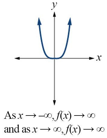
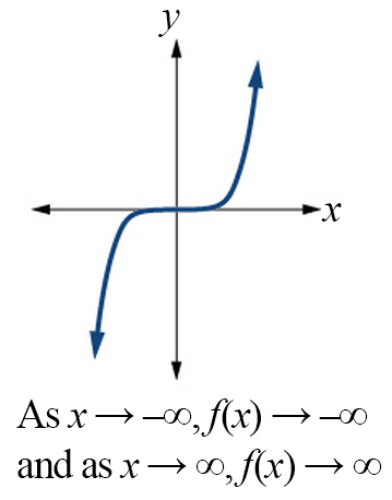
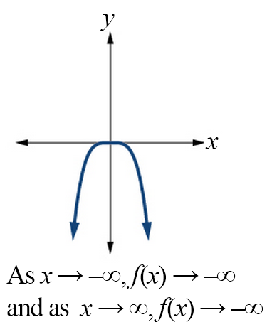
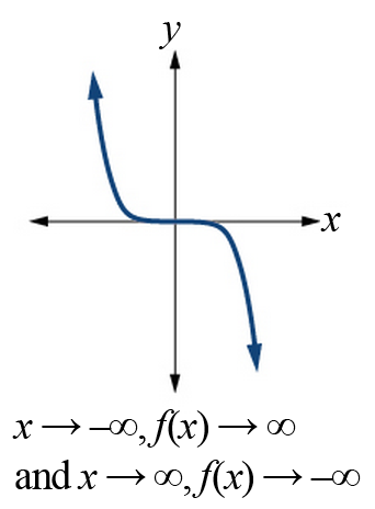
The table below shows the end behavior of power functions of the form [latex]f\left(x\right)=a{x}^{n}[/latex] where [latex]n[/latex] is a non-negative integer depending on the power and the constant.
| Even Power | Odd Power | |
|---|---|---|
| Positive Constant
a > 0 |
 |
 |
| Negative Constant
a < 0 |
 |
 |
How To: Given a power function [latex]f\left(x\right)=a{x}^{n}[/latex] where [latex]n[/latex] is a non-negative integer, identify the end behavior.
- Determine whether the power is even or odd.
- Determine whether the constant is positive or negative.
- Use the above graphs to identify the end behavior.
Example: Identifying the End Behavior of a Power Function
Describe the end behavior of the graph of [latex]f\left(x\right)={x}^{8}[/latex].

Example: Identifying the End Behavior of a Power Function
Describe the end behavior of the graph of [latex]f\left(x\right)=-{x}^{9}[/latex].

Try It
Describe in words and symbols the end behavior of [latex]f\left(x\right)=-5{x}^{4}[/latex].
End Behavior of Polynomial Functions
Identifying Polynomial Functions
An oil pipeline bursts in the Gulf of Mexico causing an oil slick in a roughly circular shape. The slick is currently 24 miles in radius, but that radius is increasing by 8 miles each week. We want to write a formula for the area covered by the oil slick by combining two functions. The radius r of the spill depends on the number of weeks w that have passed. This relationship is linear.
[latex]r\left(w\right)=24+8w[/latex]
We can combine this with the formula for the area A of a circle.
[latex]A\left(r\right)=\pi {r}^{2}[/latex]
Composing these functions gives a formula for the area in terms of weeks.
[latex]\begin{array}{l}A\left(w\right)=A\left(r\left(w\right)\right)\\ A\left(w\right)=A\left(24+8w\right)\\ A\left(w\right)=\pi {\left(24+8w\right)}^{2}\end{array}[/latex]
Multiplying gives the formula below.
[latex]A\left(w\right)=576\pi +384\pi w+64\pi {w}^{2}[/latex]
This formula is an example of a polynomial function. A polynomial function consists of either zero or the sum of a finite number of non-zero terms, each of which is a product of a number, called the coefficient of the term, and a variable raised to a non-negative integer power.
A General Note: Polynomial Functions
Let n be a non-negative integer. A polynomial function is a function that can be written in the form
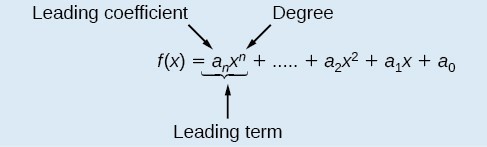
[latex]f\left(x\right)={a}_{n}{x}^{n}+\dots+{a}_{2}{x}^{2}+{a}_{1}x+{a}_{0}[/latex]
This is called the general form of a polynomial function. Each [latex]{a}_{i}[/latex] is a coefficient and can be any real number. Each product [latex]{a}_{i}{x}^{i}[/latex] is a term of a polynomial function.
Example: Identifying Polynomial Functions
Which of the following are polynomial functions?
[latex]\begin{array}{c}f\left(x\right)=2{x}^{3}\cdot 3x+4\hfill \\ g\left(x\right)=-x\left({x}^{2}-4\right)\hfill \\ h\left(x\right)=5\sqrt{x}+2\hfill \end{array}[/latex]
Try It
Defining the Degree and Leading Coefficient of a Polynomial Function
Because of the form of a polynomial function, we can see an infinite variety in the number of terms and the power of the variable. Although the order of the terms in the polynomial function is not important for performing operations, we typically arrange the terms in descending order based on the power on the variable. This is called writing a polynomial in general or standard form. The degree of the polynomial is the highest power of the variable that occurs in the polynomial; it is the power of the first variable if the function is in general form. The leading term is the term containing the variable with the highest power, also called the term with the highest degree. The leading coefficient is the coefficient of the leading term.
A General Note: Terminology of Polynomial Functions
We often rearrange polynomials so that the powers on the variable are descending.
When a polynomial is written in this way, we say that it is in general form.
How To: Given a polynomial function, identify the degree and leading coefficient
- Find the highest power of x to determine the degree of the function.
- Identify the term containing the highest power of x to find the leading term.
- The leading coefficient is the coefficient of the leading term.
Example: Identifying the Degree and Leading Coefficient of a Polynomial Function
Identify the degree, leading term, and leading coefficient of the following polynomial functions.
[latex]\begin{array}{l} f\left(x\right)=3+2{x}^{2}-4{x}^{3} \\g\left(t\right)=5{t}^{5}-2{t}^{3}+7t\\h\left(p\right)=6p-{p}^{3}-2\end{array}[/latex]
Try It
Identify the degree, leading term, and leading coefficient of the polynomial [latex]f\left(x\right)=4{x}^{2}-{x}^{6}+2x - 6[/latex].
In the following video, we show more examples of how to determine the degree, leading term, and leading coefficient of a polynomial.
Identifying End Behavior of Polynomial Functions
Knowing the leading coefficient and degree of a polynomial function is useful when predicting its end behavior. To determine its end behavior, look at the leading term of the polynomial function. Because the power of the leading term is the highest, that term will grow significantly faster than the other terms as x gets very large or very small, so its behavior will dominate the graph. For any polynomial, the end behavior of the polynomial will match the end behavior of the term of highest degree.
| Polynomial Function | Leading Term | Graph of Polynomial Function |
|---|---|---|
| [latex]f\left(x\right)=5{x}^{4}+2{x}^{3}-x - 4[/latex] | [latex]5{x}^{4}[/latex] | 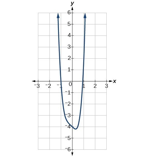 |
| [latex]f\left(x\right)=-2{x}^{6}-{x}^{5}+3{x}^{4}+{x}^{3}[/latex] | [latex]-2{x}^{6}[/latex] | 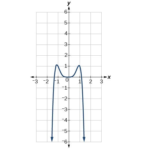 |
| [latex]f\left(x\right)=3{x}^{5}-4{x}^{4}+2{x}^{2}+1[/latex] | [latex]3{x}^{5}[/latex] | 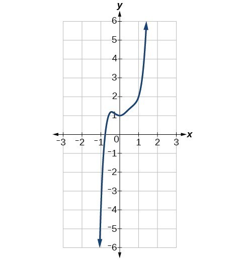 |
| [latex]f\left(x\right)=-6{x}^{3}+7{x}^{2}+3x+1[/latex] | [latex]-6{x}^{3}[/latex] | 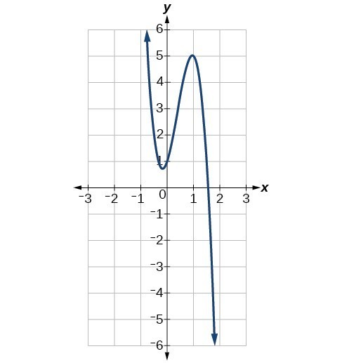 |
Example: Identifying End Behavior and Degree of a Polynomial Function
Describe the end behavior and determine a possible degree of the polynomial function in the graph below.
In the following video, we show more examples that summarize the end behavior of polynomial functions and which components of the function contribute to it.
Try It
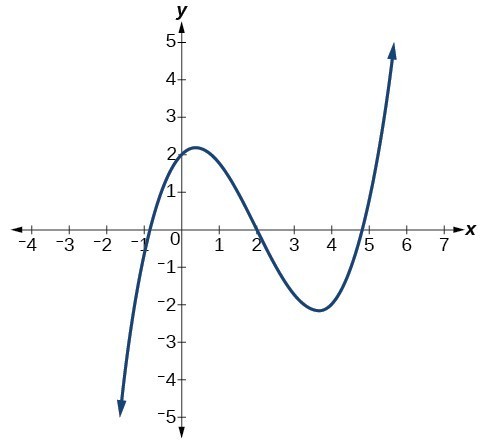
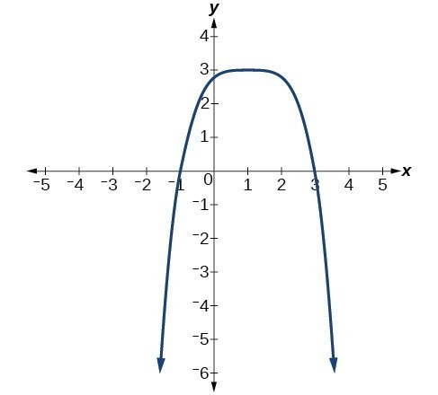
Describe the end behavior of the polynomial function in the graph below.
Example: Identifying End Behavior and Degree of a Polynomial Function
Given the function [latex]f\left(x\right)=-3{x}^{2}\left(x - 1\right)\left(x+4\right)[/latex], express the function as a polynomial in general form and determine the leading term, degree, and end behavior of the function.
Try It
Given the function [latex]f\left(x\right)=0.2\left(x - 2\right)\left(x+1\right)\left(x - 5\right)[/latex], express the function as a polynomial in general form and determine the leading term, degree, and end behavior of the function.
Local Behavior of Polynomial Functions
Identifying Local Behavior of Polynomial Functions
In addition to the end behavior of polynomial functions, we are also interested in what happens in the “middle” of the function. In particular, we are interested in locations where graph behavior changes. A turning point is a point at which the function values change from increasing to decreasing or decreasing to increasing.
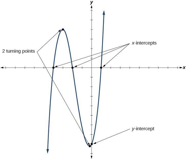
We are also interested in the intercepts. As with all functions, the y-intercept is the point at which the graph intersects the vertical axis. The point corresponds to the coordinate pair in which the input value is zero. Because a polynomial is a function, only one output value corresponds to each input value so there can be only one y-intercept [latex]\left(0,{a}_{0}\right)[/latex]. The x-intercepts occur at the input values that correspond to an output value of zero. It is possible to have more than one x-intercept.
A General Note: Intercepts and Turning Points of Polynomial Functions
- A turning point of a graph is a point where the graph changes from increasing to decreasing or decreasing to increasing.
- The y-intercept is the point where the function has an input value of zero.
- The x-intercepts are the points where the output value is zero.
- A polynomial of degree n will have, at most, n x-intercepts and n – 1 turning points.
Determining the Number of Turning Points and Intercepts from the Degree of the Polynomial
A continuous function has no breaks in its graph: the graph can be drawn without lifting the pen from the paper. A smooth curve is a graph that has no sharp corners. The turning points of a smooth graph must always occur at rounded curves. The graphs of polynomial functions are both continuous and smooth.
The degree of a polynomial function helps us to determine the number of x-intercepts and the number of turning points. A polynomial function of nth degree is the product of n factors, so it will have at most n roots or zeros, or x-intercepts. The graph of the polynomial function of degree n must have at most n – 1 turning points. This means the graph has at most one fewer turning point than the degree of the polynomial or one fewer than the number of factors.
Example: Determining the Number of Intercepts and Turning Points of a Polynomial
Without graphing the function, determine the local behavior of the function by finding the maximum number of x-intercepts and turning points for [latex]f\left(x\right)=-3{x}^{10}+4{x}^{7}-{x}^{4}+2{x}^{3}[/latex].
The following video gives a 5 minute lesson on how to determine the number of intercepts and turning points of a polynomial function given its degree.
Try It
Without graphing the function, determine the maximum number of x-intercepts and turning points for [latex]f\left(x\right)=108 - 13{x}^{9}-8{x}^{4}+14{x}^{12}+2{x}^{3}[/latex]
How To: Given a polynomial function, determine the intercepts
- Determine the y-intercept by setting [latex]x=0[/latex] and finding the corresponding output value.
- Determine the x-intercepts by setting the function equal to zero and solving for the input values.
Using the Principle of Zero Products to Find the Roots of a Polynomial in Factored Form
The Principle of Zero Products states that if the product of n numbers is 0, then at least one of the factors is 0. If [latex]ab=0[/latex], then either [latex]a=0[/latex] or [latex]b=0[/latex], or both a and b are 0. We will use this idea to find the zeros of a polynomial that is either in factored form or can be written in factored form. For example, the polynomial
[latex]P(x)=(x-4)^2(x+1)(x-7)[/latex]
is in factored form. In the following examples, we will show the process of factoring a polynomial and calculating its x and y-intercepts.
Example: Determining the Intercepts of a Polynomial Function
Given the polynomial function [latex]f\left(x\right)=\left(x - 2\right)\left(x+1\right)\left(x - 4\right)[/latex], written in factored form for your convenience, determine the y and x-intercepts.

Example: Determining the Intercepts of a Polynomial Function BY Factoring
Given the polynomial function [latex]f\left(x\right)={x}^{4}-4{x}^{2}-45[/latex], determine the y and x-intercepts.

Try It
Given the polynomial function [latex]f\left(x\right)=2{x}^{3}-6{x}^{2}-20x[/latex], determine the y and x-intercepts.
The Whole Picture
Now we can bring the two concepts of turning points and intercepts together to get a general picture of the behavior of polynomial functions. These types of analyses on polynomials developed before the advent of mass computing as a way to quickly understand the general behavior of a polynomial function. We now have a quick way, with computers, to graph and calculate important characteristics of polynomials that once took a lot of algebra.
In the first example, we will determine the least degree of a polynomial based on the number of turning points and intercepts.
Example: Drawing Conclusions about a Polynomial Function from Its Graph
Given the graph of the polynomial function below, determine the least possible degree of the polynomial and whether it is even or odd. Use end behavior, the number of intercepts, and the number of turning points to help you.
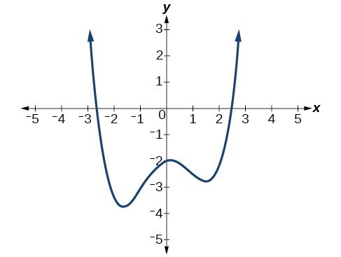

Now you try to determine the least possible degree of a polynomial given its graph.
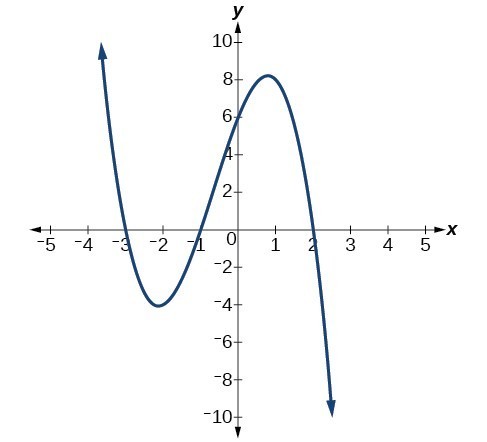
Try It
Given the graph of the polynomial function below, determine the least possible degree of the polynomial and whether it is even or odd. Use end behavior, the number of intercepts, and the number of turning points to help you.
Now we will show that you can also determine the least possible degree and number of turning points of a polynomial function given in factored form.
Example: Drawing Conclusions about a Polynomial Function from ITS Factors
Given the function [latex]f\left(x\right)=-4x\left(x+3\right)\left(x - 4\right)[/latex], determine the local behavior.
Now it is your turn to determine the local behavior of a polynomial given in factored form.
Try It
Given the function [latex]f\left(x\right)=0.2\left(x - 2\right)\left(x+1\right)\left(x - 5\right)[/latex], determine the local behavior.
Key Equations
| general form of a polynomial function | [latex]f\left(x\right)={a}_{n}{x}^{n}+\dots+{a}_{2}{x}^{2}+{a}_{1}x+{a}_{0}[/latex] |
Key Concepts
- A power function is a variable base raised to a number power.
- The behavior of a graph as the input decreases beyond bound and increases beyond bound is called the end behavior.
- The end behavior depends on whether the power is even or odd.
- A polynomial function is the sum of terms, each of which consists of a transformed power function with non-negative integer powers.
- The degree of a polynomial function is the highest power of the variable that occurs in a polynomial. The term containing the highest power of the variable is called the leading term. The coefficient of the leading term is called the leading coefficient.
- The end behavior of a polynomial function is the same as the end behavior of the power function represented by the leading term of the function.
- A polynomial of degree n will have at most n x-intercepts and at most n – 1 turning points.
Glossary
- coefficient
- a nonzero real number multiplied by a variable raised to an exponent
- continuous function
- a function whose graph can be drawn without lifting the pen from the paper because there are no breaks in the graph
- degree
- the highest power of the variable that occurs in a polynomial
- end behavior
- the behavior of the graph of a function as the input decreases without bound and increases without bound
- leading coefficient
- the coefficient of the leading term
- leading term
- the term containing the highest power of the variable
- polynomial function
- a function that consists of either zero or the sum of a finite number of non-zero terms, each of which is a product of a number, called the coefficient of the term, and a variable raised to a non-negative integer power.
- power function
- a function that can be represented in the form [latex]f\left(x\right)=a{x}^{n}[/latex] where a is a constant, the base is a variable, and the exponent is n, is a smooth curve represented by a graph with no sharp corners
- term of a polynomial function
- any [latex]{a}_{i}{x}^{i}[/latex] of a polynomial function in the form [latex]f\left(x\right)={a}_{n}{x}^{n}+\dots+{a}_{2}{x}^{2}+{a}_{1}x+{a}_{0}[/latex]
- turning point
- the location where the graph of a function changes direction
Candela Citations
- Revision and Adaptation. Provided by: Lumen Learning. License: CC BY: Attribution
- Degree, Leading Term, and Leading Coefficient of a Polynomial Function . Authored by: James Sousa (Mathispower4u.com) for Lumen Learning. Located at: https://youtu.be/F_G_w82s0QA. License: CC BY: Attribution
- College Algebra. Authored by: Abramson, Jay et al.. Provided by: OpenStax. Located at: http://cnx.org/contents/9b08c294-057f-4201-9f48-5d6ad992740d@5.2. License: CC BY: Attribution. License Terms: Download for free at http://cnx.org/contents/9b08c294-057f-4201-9f48-5d6ad992740d@5.2
- Question ID 69337. Authored by: Roy Shahbazian. License: CC BY: Attribution. License Terms: IMathAS Community License CC-BY + GPL
- Question ID 15940, 15937. Authored by: James Sousa. License: CC BY: Attribution. License Terms: IMathAS Community License CC-BY + GPL
- Ex: End Behavior or Long Run Behavior of Functions.. Authored by: James Sousa (Mathispower4u.com) . Located at: https://youtu.be/Krjd_vU4Uvg. License: CC BY: Attribution
- Question ID 48358. Authored by: Wicks, Edward. License: CC BY: Attribution. License Terms: IMathAS Community License CC-BY + GPL
- Question ID 121444, 123739. Provided by: Lumen Learning. License: CC BY: Attribution. License Terms: IMathAS Community License CC-BY + GPL
- Summary of End Behavior or Long Run Behavior of Polynomial Functions . Authored by: James Sousa (Mathispower4u.com). Located at: https://youtu.be/y78Dpr9LLN0. License: CC BY: Attribution
- Turning Points and X-Intercepts of a Polynomial Function. Authored by: Sousa, James (Mathispower4u). Located at: https://youtu.be/9WW0EetLD4Q. License: CC BY: Attribution