Learning Outcomes
- Determine whether a graph has an Euler path and/ or circuit
- Use Fleury’s algorithm to find an Euler circuit
- Add edges to a graph to create an Euler circuit if one doesn’t exist
- Identify whether a graph has a Hamiltonian circuit or path
- Find the optimal Hamiltonian circuit for a graph using the brute force algorithm, the nearest neighbor algorithm, and the sorted edges algorithm
- Identify a connected graph that is a spanning tree
- Use Kruskal’s algorithm to form a spanning tree, and a minimum cost spanning tree
In the next lesson, we will investigate specific kinds of paths through a graph called Euler paths and circuits. Euler paths are an optimal path through a graph. They are named after him because it was Euler who first defined them.
By counting the number of vertices of a graph, and their degree we can determine whether a graph has an Euler path or circuit. We will also learn another algorithm that will allow us to find an Euler circuit once we determine that a graph has one.
Euler Circuits
In the first section, we created a graph of the Königsberg bridges and asked whether it was possible to walk across every bridge once. Because Euler first studied this question, these types of paths are named after him.
Euler Path
An Euler path is a path that uses every edge in a graph with no repeats. Being a path, it does not have to return to the starting vertex.
Example
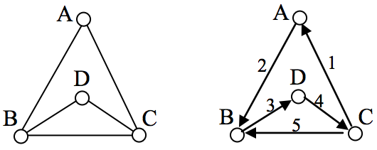
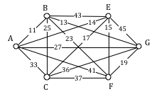
In the graph shown below, there are several Euler paths. One such path is CABDCB. The path is shown in arrows to the right, with the order of edges numbered.
Euler Circuit
An Euler circuit is a circuit that uses every edge in a graph with no repeats. Being a circuit, it must start and end at the same vertex.
Example
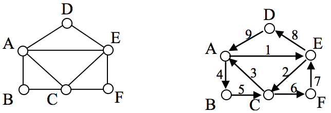
The graph below has several possible Euler circuits. Here’s a couple, starting and ending at vertex A: ADEACEFCBA and AECABCFEDA. The second is shown in arrows.
Look back at the example used for Euler paths—does that graph have an Euler circuit? A few tries will tell you no; that graph does not have an Euler circuit. When we were working with shortest paths, we were interested in the optimal path. With Euler paths and circuits, we’re primarily interested in whether an Euler path or circuit exists.
Why do we care if an Euler circuit exists? Think back to our housing development lawn inspector from the beginning of the chapter. The lawn inspector is interested in walking as little as possible. The ideal situation would be a circuit that covers every street with no repeats. That’s an Euler circuit! Luckily, Euler solved the question of whether or not an Euler path or circuit will exist.
Euler’s Path and Circuit Theorems
A graph will contain an Euler path if it contains at most two vertices of odd degree.
A graph will contain an Euler circuit if all vertices have even degree
Example
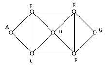
In the graph below, vertices A and C have degree 4, since there are 4 edges leading into each vertex. B is degree 2, D is degree 3, and E is degree 1. This graph contains two vertices with odd degree (D and E) and three vertices with even degree (A, B, and C), so Euler’s theorems tell us this graph has an Euler path, but not an Euler circuit.
Example
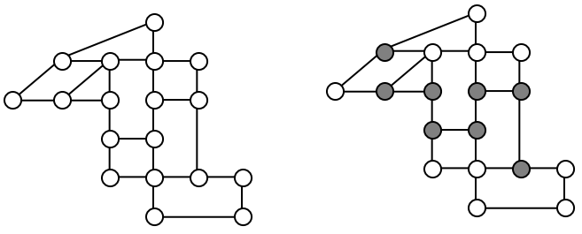
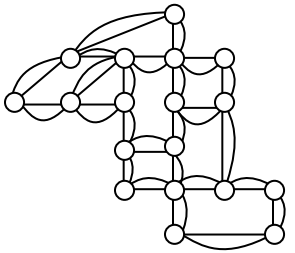
Is there an Euler circuit on the housing development lawn inspector graph we created earlier in the chapter? All the highlighted vertices have odd degree. Since there are more than two vertices with odd degree, there are no Euler paths or Euler circuits on this graph. Unfortunately our lawn inspector will need to do some backtracking.
Example
When it snows in the same housing development, the snowplow has to plow both sides of every street. For simplicity, we’ll assume the plow is out early enough that it can ignore traffic laws and drive down either side of the street in either direction. This can be visualized in the graph by drawing two edges for each street, representing the two sides of the street.
Notice that every vertex in this graph has even degree, so this graph does have an Euler circuit.
The following video gives more examples of how to determine an Euler path, and an Euler Circuit for a graph.
Fleury’s Algorithm
Fleury’s Algorithm
Example
Find an Euler Circuit on this graph using Fleury’s algorithm, starting at vertex A.

Try It
Does the graph below have an Euler Circuit? If so, find one.
The following video presents more examples of using Fleury’s algorithm to find an Euler Circuit.
Eulerization and the Chinese Postman Problem
Not every graph has an Euler path or circuit, yet our lawn inspector still needs to do her inspections. Her goal is to minimize the amount of walking she has to do. In order to do that, she will have to duplicate some edges in the graph until an Euler circuit exists.
Eulerization
Eulerization is the process of adding edges to a graph to create an Euler circuit on a graph. To eulerize a graph, edges are duplicated to connect pairs of vertices with odd degree. Connecting two odd degree vertices increases the degree of each, giving them both even degree. When two odd degree vertices are not directly connected, we can duplicate all edges in a path connecting the two.
Note that we can only duplicate edges, not create edges where there wasn’t one before. Duplicating edges would mean walking or driving down a road twice, while creating an edge where there wasn’t one before is akin to installing a new road!
Example
For the rectangular graph shown, three possible eulerizations are shown. Notice in each of these cases the vertices that started with odd degrees have even degrees after eulerization, allowing for an Euler circuit.


In the example above, you’ll notice that the last eulerization required duplicating seven edges, while the first two only required duplicating five edges. If we were eulerizing the graph to find a walking path, we would want the eulerization with minimal duplications. If the edges had weights representing distances or costs, then we would want to select the eulerization with the minimal total added weight.
Try It now
Eulerize the graph shown, then find an Euler circuit on the eulerized graph.

Example
Looking again at the graph for our lawn inspector from Examples 1 and 8, the vertices with odd degree are shown highlighted. With eight vertices, we will always have to duplicate at least four edges. In this case, we need to duplicate five edges since two odd degree vertices are not directly connected. Without weights we can’t be certain this is the eulerization that minimizes walking distance, but it looks pretty good.


The problem of finding the optimal eulerization is called the Chinese Postman Problem, a name given by an American in honor of the Chinese mathematician Mei-Ko Kwan who first studied the problem in 1962 while trying to find optimal delivery routes for postal carriers. This problem is important in determining efficient routes for garbage trucks, school buses, parking meter checkers, street sweepers, and more.
Unfortunately, algorithms to solve this problem are fairly complex. Some simpler cases are considered in the exercises
The following video shows another view of finding an Eulerization of the lawn inspector problem.
Hamiltonian Circuits
The Traveling Salesman Problem
In the last section, we considered optimizing a walking route for a postal carrier. How is this different than the requirements of a package delivery driver? While the postal carrier needed to walk down every street (edge) to deliver the mail, the package delivery driver instead needs to visit every one of a set of delivery locations. Instead of looking for a circuit that covers every edge once, the package deliverer is interested in a circuit that visits every vertex once.
Hamiltonian Circuits and Paths
A Hamiltonian circuit is a circuit that visits every vertex once with no repeats. Being a circuit, it must start and end at the same vertex. A Hamiltonian path also visits every vertex once with no repeats, but does not have to start and end at the same vertex.
Hamiltonian circuits are named for William Rowan Hamilton who studied them in the 1800’s.
Example
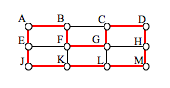
One Hamiltonian circuit is shown on the graph below. There are several other Hamiltonian circuits possible on this graph. Notice that the circuit only has to visit every vertex once; it does not need to use every edge.
This circuit could be notated by the sequence of vertices visited, starting and ending at the same vertex: ABFGCDHMLKJEA. Notice that the same circuit could be written in reverse order, or starting and ending at a different vertex.
Unlike with Euler circuits, there is no nice theorem that allows us to instantly determine whether or not a Hamiltonian circuit exists for all graphs.[1]
Example
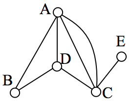
Does a Hamiltonian path or circuit exist on the graph below?

We can see that once we travel to vertex E there is no way to leave without returning to C, so there is no possibility of a Hamiltonian circuit. If we start at vertex E we can find several Hamiltonian paths, such as ECDAB and ECABD
Try It
With Hamiltonian circuits, our focus will not be on existence, but on the question of optimization; given a graph where the edges have weights, can we find the optimal Hamiltonian circuit; the one with lowest total weight.
Watch this video to see the examples above worked out.
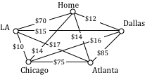
This problem is called the Traveling salesman problem (TSP) because the question can be framed like this: Suppose a salesman needs to give sales pitches in four cities. He looks up the airfares between each city, and puts the costs in a graph. In what order should he travel to visit each city once then return home with the lowest cost?
To answer this question of how to find the lowest cost Hamiltonian circuit, we will consider some possible approaches. The first option that might come to mind is to just try all different possible circuits.
question can be framed like this: Suppose a salesman needs to give sales pitches in four cities. He looks up the airfares between each city, and puts the costs in a graph. In what order should he travel to visit each city once then return home with the lowest cost?
To answer this question of how to find the lowest cost Hamiltonian circuit, we will consider some possible approaches. The first option that might come to mind is to just try all different possible circuits.
Brute Force Algorithm (a.k.a. exhaustive search)
1. List all possible Hamiltonian circuits
2. Find the length of each circuit by adding the edge weights
3. Select the circuit with minimal total weight.
Example
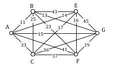
Apply the Brute force algorithm to find the minimum cost Hamiltonian circuit on the graph below.

To apply the Brute force algorithm, we list all possible Hamiltonian circuits and calculate their weight:
| Circuit | Weight |
| ABCDA | 4+13+8+1 = 26 |
| ABDCA | 4+9+8+2 = 23 |
| ACBDA | 2+13+9+1 = 25 |
Note: These are the unique circuits on this graph. All other possible circuits are the reverse of the listed ones or start at a different vertex, but result in the same weights.
From this we can see that the second circuit, ABDCA, is the optimal circuit.
Watch these examples worked again in the following video.
Try It
The Brute force algorithm is optimal; it will always produce the Hamiltonian circuit with minimum weight. Is it efficient? To answer that question, we need to consider how many Hamiltonian circuits a graph could have. For simplicity, let’s look at the worst-case possibility, where every vertex is connected to every other vertex. This is called a complete graph.
Suppose we had a complete graph with five vertices like the air travel graph above. From Seattle there are four cities we can visit first. From each of those, there are three choices. From each of those cities, there are two possible cities to visit next. There is then only one choice for the last city before returning home.
This can be shown visually:

Counting the number of routes, we can see thereare [latex]4\cdot{3}\cdot{2}\cdot{1}[/latex] routes. For six cities there would be [latex]5\cdot{4}\cdot{3}\cdot{2}\cdot{1}[/latex] routes.
Number of Possible Circuits
For N vertices in a complete graph, there will be [latex](n-1)!=(n-1)(n-2)(n-3)\dots{3}\cdot{2}\cdot{1}[/latex] routes. Half of these are duplicates in reverse order, so there are [latex]\frac{(n-1)!}{2}[/latex] unique circuits.
The exclamation symbol, !, is read “factorial” and is shorthand for the product shown.
Example
How many circuits would a complete graph with 8 vertices have?
A complete graph with 8 vertices would have = 5040 possible Hamiltonian circuits. Half of the circuits are duplicates of other circuits but in reverse order, leaving 2520 unique routes.
While this is a lot, it doesn’t seem unreasonably huge. But consider what happens as the number of cities increase:
| Cities | Unique Hamiltonian Circuits |
| 9 | 8!/2 = 20,160 |
| 10 | 9!/2 = 181,440 |
| 11 | 10!/2 = 1,814,400 |
| 15 | 14!/2 = 43,589,145,600 |
| 20 | 19!/2 = 60,822,550,204,416,000 |
Watch these examples worked again in the following video.
As you can see the number of circuits is growing extremely quickly. If a computer looked at one billion circuits a second, it would still take almost two years to examine all the possible circuits with only 20 cities! Certainly Brute Force is not an efficient algorithm.
Nearest Neighbor Algorithm (NNA)
1. Select a starting point.
2. Move to the nearest unvisited vertex (the edge with smallest weight).
3. Repeat until the circuit is complete.
Unfortunately, no one has yet found an efficient and optimal algorithm to solve the TSP, and it is very unlikely anyone ever will. Since it is not practical to use brute force to solve the problem, we turn instead to heuristic algorithms; efficient algorithms that give approximate solutions. In other words, heuristic algorithms are fast, but may or may not produce the optimal circuit.
Example
Consider our earlier graph, shown to the right.
Starting at vertex A, the nearest neighbor is vertex D with a weight of 1.
From D, the nearest neighbor is C, with a weight of 8.
From C, our only option is to move to vertex B, the only unvisited vertex, with a cost of 13.
From B we return to A with a weight of 4.
The resulting circuit is ADCBA with a total weight of [latex]1+8+13+4 = 26[/latex].
Watch the example worked out in the following video.
We ended up finding the worst circuit in the graph! What happened? Unfortunately, while it is very easy to implement, the NNA is a greedy algorithm, meaning it only looks at the immediate decision without considering the consequences in the future. In this case, following the edge AD forced us to use the very expensive edge BC later.
Example
Consider again our salesman. Starting in Seattle, the nearest neighbor (cheapest flight) is to LA, at a cost of $70. From there:
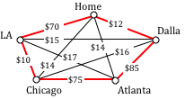
LA to Chicago: $100
Chicago to Atlanta: $75
Atlanta to Dallas: $85
Dallas to Seattle: $120
Total cost: $450
In this case, nearest neighbor did find the optimal circuit.
Watch this example worked out again in this video.
Going back to our first example, how could we improve the outcome? One option would be to redo the nearest neighbor algorithm with a different starting point to see if the result changed. Since nearest neighbor is so fast, doing it several times isn’t a big deal.
Example
We will revisit the graph from Example 17.
Starting at vertex A resulted in a circuit with weight 26.
Starting at vertex B, the nearest neighbor circuit is BADCB with a weight of 4+1+8+13 = 26. This is the same circuit we found starting at vertex A. No better.
Starting at vertex C, the nearest neighbor circuit is CADBC with a weight of 2+1+9+13 = 25. Better!
Starting at vertex D, the nearest neighbor circuit is DACBA. Notice that this is actually the same circuit we found starting at C, just written with a different starting vertex.
The RNNA was able to produce a slightly better circuit with a weight of 25, but still not the optimal circuit in this case. Notice that even though we found the circuit by starting at vertex C, we could still write the circuit starting at A: ADBCA or ACBDA.
Try It
The table below shows the time, in milliseconds, it takes to send a packet of data between computers on a network. If data needed to be sent in sequence to each computer, then notification needed to come back to the original computer, we would be solving the TSP. The computers are labeled A-F for convenience.
| A | B | C | D | E | F | |
| A | — | 44 | 34 | 12 | 40 | 41 |
| B | 44 | — | 31 | 43 | 24 | 50 |
| C | 34 | 31 | — | 20 | 39 | 27 |
| D | 12 | 43 | 20 | — | 11 | 17 |
| E | 40 | 24 | 39 | 11 | — | 42 |
| F | 41 | 50 | 27 | 17 | 42 | — |
a. Find the circuit generated by the NNA starting at vertex B.
b. Find the circuit generated by the RNNA.
While certainly better than the basic NNA, unfortunately, the RNNA is still greedy and will produce very bad results for some graphs. As an alternative, our next approach will step back and look at the “big picture” – it will select first the edges that are shortest, and then fill in the gaps.
Example
Using the four vertex graph from earlier, we can use the Sorted Edges algorithm.
The cheapest edge is AD, with a cost of 1. We highlight that edge to mark it selected.
The next shortest edge is AC, with a weight of 2, so we highlight that edge.


For the third edge, we’d like to add AB, but that would give vertex A degree 3, which is not allowed in a Hamiltonian circuit. The next shortest edge is CD, but that edge would create a circuit ACDA that does not include vertex B, so we reject that edge. The next shortest edge is BD, so we add that edge to the graph.

BAD

BAD

OK
We then add the last edge to complete the circuit: ACBDA with weight 25.
Notice that the algorithm did not produce the optimal circuit in this case; the optimal circuit is ACDBA with weight 23.

While the Sorted Edge algorithm overcomes some of the shortcomings of NNA, it is still only a heuristic algorithm, and does not guarantee the optimal circuit.
Example
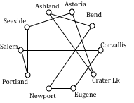
Your teacher’s band, Derivative Work, is doing a bar tour in Oregon. The driving distances are shown below. Plan an efficient route for your teacher to visit all the cities and return to the starting location. Use NNA starting at Portland, and then use Sorted Edges.
| Ashland | Astoria | Bend | Corvallis | Crater Lake | Eugene | Newport | Portland | Salem | Seaside | |
| Ashland | – | 374 | 200 | 223 | 108 | 178 | 252 | 285 | 240 | 356 |
| Astoria | 374 | – | 255 | 166 | 433 | 199 | 135 | 95 | 136 | 17 |
| Bend | 200 | 255 | – | 128 | 277 | 128 | 180 | 160 | 131 | 247 |
| Corvallis | 223 | 166 | 128 | – | 430 | 47 | 52 | 84 | 40 | 155 |
| Crater Lake | 108 | 433 | 277 | 430 | – | 453 | 478 | 344 | 389 | 423 |
| Eugene | 178 | 199 | 128 | 47 | 453 | – | 91 | 110 | 64 | 181 |
| Newport | 252 | 135 | 180 | 52 | 478 | 91 | – | 114 | 83 | 117 |
| Portland | 285 | 95 | 160 | 84 | 344 | 110 | 114 | – | 47 | 78 |
| Salem | 240 | 136 | 131 | 40 | 389 | 64 | 83 | 47 | – | 118 |
| Seaside | 356 | 17 | 247 | 155 | 423 | 181 | 117 | 78 | 118 | – |
To see the entire table, scroll to the right
Using NNA with a large number of cities, you might find it helpful to mark off the cities as they’re visited to keep from accidently visiting them again. Looking in the row for Portland, the smallest distance is 47, to Salem. Following that idea, our circuit will be:
Portland to Salem 47
Salem to Corvallis 40
Corvallis to Eugene 47
Eugene to Newport 91
Newport to Seaside 117
Seaside to Astoria 17
Astoria to Bend 255
Bend to Ashland 200
Ashland to Crater Lake 108
Crater Lake to Portland 344
Total trip length: 1266 miles
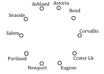
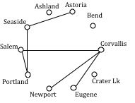
Using Sorted Edges, you might find it helpful to draw an empty graph, perhaps by drawing vertices in a circular pattern. Adding edges to the graph as you select them will help you visualize any circuits or vertices with degree 3.
We start adding the shortest edges:
Seaside to Astoria 17 miles
Corvallis to Salem 40 miles
Portland to Salem 47 miles
Corvallis to Eugene 47 miles
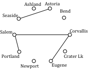
The graph after adding these edges is shown to the right. The next shortest edge is from Corvallis to Newport at 52 miles, but adding that edge would give Corvallis degree 3.
Continuing on, we can skip over any edge pair that contains Salem or Corvallis, since they both already have degree 2.
Portland to Seaside 78 miles
Eugene to Newport 91 miles
Portland to Astoria (reject – closes circuit)
Ashland to Crater Lk 108 miles
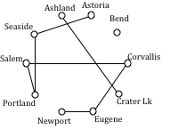
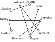
The graph after adding these edges is shown to the right. At this point, we can skip over any edge pair that contains Salem, Seaside, Eugene, Portland, or Corvallis since they already have degree 2.
Newport to Astoria (reject – closes circuit)
Newport to Bend 180 miles
Bend to Ashland 200 miles
At this point the only way to complete the circuit is to add:
Crater Lk to Astoria 433 miles. The final circuit, written to start at Portland, is:
Portland, Salem, Corvallis, Eugene, Newport, Bend, Ashland, Crater Lake, Astoria, Seaside, Portland. Total trip length: 1241 miles.
While better than the NNA route, neither algorithm produced the optimal route. The following route can make the tour in 1069 miles:
Portland, Astoria, Seaside, Newport, Corvallis, Eugene, Ashland, Crater Lake, Bend, Salem, Portland
Watch the example of nearest neighbor algorithm for traveling from city to city using a table worked out in the video below.
In the next video we use the same table, but use sorted edges to plan the trip.
Try It
Find the circuit produced by the Sorted Edges algorithm using the graph below.
Spanning Trees
A company requires reliable internet and phone connectivity between their five offices (named A, B, C, D, and E for simplicity) in New York, so they decide to lease dedicated lines from the phone company. The phone company will charge for each link made. The costs, in thousands of dollars per year, are shown in the graph.
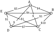
In this case, we don’t need to find a circuit, or even a specific path; all we need to do is make sure we can make a call from any office to any other. In other words, we need to be sure there is a path from any vertex to any other vertex.
Spanning Tree
A spanning tree is a connected graph using all vertices in which there are no circuits.
In other words, there is a path from any vertex to any other vertex, but no circuits.
Some examples of spanning trees are shown below. Notice there are no circuits in the trees, and it is fine to have vertices with degree higher than two.

Usually we have a starting graph to work from, like in the phone example above. In this case, we form our spanning tree by finding a subgraph – a new graph formed using all the vertices but only some of the edges from the original graph. No edges will be created where they didn’t already exist.
Of course, any random spanning tree isn’t really what we want. We want the minimum cost spanning tree (MCST).
Minimum Cost Spanning Tree (MCST)
The minimum cost spanning tree is the spanning tree with the smallest total edge weight.
A nearest neighbor style approach doesn’t make as much sense here since we don’t need a circuit, so instead we will take an approach similar to sorted edges.
Kruskal’s Algorithm
- Select the cheapest unused edge in the graph.
- Repeat step 1, adding the cheapest unused edge, unless:
- adding the edge would create a circuit
Repeat until a spanning tree is formed
Example
Using our phone line graph from above, begin adding edges:
AB $4 OK
AE $5 OK
BE $6 reject – closes circuit ABEA
DC $7 OK
AC $8 OK
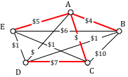
At this point we stop – every vertex is now connected, so we have formed a spanning tree with cost $24 thousand a year.
Remarkably, Kruskal’s algorithm is both optimal and efficient; we are guaranteed to always produce the optimal MCST.
Example
The power company needs to lay updated distribution lines connecting the ten Oregon cities below to the power grid. How can they minimize the amount of new line to lay?
| Ashland | Astoria | Bend | Corvallis | Crater Lake | Eugene | Newport | Portland | Salem | Seaside | |
| Ashland | – | 374 | 200 | 223 | 108 | 178 | 252 | 285 | 240 | 356 |
| Astoria | 374 | – | 255 | 166 | 433 | 199 | 135 | 95 | 136 | 17 |
| Bend | 200 | 255 | – | 128 | 277 | 128 | 180 | 160 | 131 | 247 |
| Corvallis | 223 | 166 | 128 | – | 430 | 47 | 52 | 84 | 40 | 155 |
| Crater Lake | 108 | 433 | 277 | 430 | – | 453 | 478 | 344 | 389 | 423 |
| Eugene | 178 | 199 | 128 | 47 | 453 | – | 91 | 110 | 64 | 181 |
| Newport | 252 | 135 | 180 | 52 | 478 | 91 | – | 114 | 83 | 117 |
| Portland | 285 | 95 | 160 | 84 | 344 | 110 | 114 | – | 47 | 78 |
| Salem | 240 | 136 | 131 | 40 | 389 | 64 | 83 | 47 | – | 118 |
| Seaside | 356 | 17 | 247 | 155 | 423 | 181 | 117 | 78 | 118 | – |
Using Kruskal’s algorithm, we add edges from cheapest to most expensive, rejecting any that close a circuit. We stop when the graph is connected.
Seaside to Astoria 17 milesCorvallis to Salem 40 miles
Portland to Salem 47 miles
Corvallis to Eugene 47 miles
Corvallis to Newport 52 miles
Salem to Eugene reject – closes circuit
Portland to Seaside 78 miles
The graph up to this point is shown below.
Continuing,
Newport to Salem reject
Corvallis to Portland reject
Eugene to Newport reject
Portland to Astoria reject
Ashland to Crater Lk 108 miles
Eugene to Portland reject
Newport to Portland reject
Newport to Seaside reject
Salem to Seaside reject
Bend to Eugene 128 miles
Bend to Salem reject
Astoria to Newport reject
Salem to Astoria reject
Corvallis to Seaside reject
Portland to Bend reject
Astoria to Corvallis reject
Eugene to Ashland 178 miles
This connects the graph. The total length of cable to lay would be 695 miles.
Watch the example above worked out in the following video, without a table.
Now we present the same example, with a table in the following video.
Try It
Find a minimum cost spanning tree on the graph below using Kruskal’s algorithm.
[1] There are some theorems that can be used in specific circumstances, such as Dirac’s theorem, which says that a Hamiltonian circuit must exist on a graph with n vertices if each vertex has degree n/2 or greater.
Candela Citations
- Revision and Adaptaion. Provided by: Lumen Learning. License: CC BY: Attribution
- Learning Outcomes and Introduction. Provided by: Lumen Learning. License: CC BY: Attribution
- Graph Theory: Euler Paths and Euler Circuits . Authored by: James Sousa (Mathispower4u.com). Located at: https://youtu.be/5M-m62qTR-s. License: CC BY: Attribution
- Math in Society. Authored by: Lippman, David. License: CC BY: Attribution
- Graph Theory: Fleury's Algorthim . Authored by: James Sousa (Mathispower4u.com). Located at: https://youtu.be/vvP4Fg4r-Ns. License: CC BY: Attribution
- Hamiltonian circuits. Authored by: OCLPhase2. Located at: https://youtu.be/lUqCtywkskU. License: CC BY: Attribution
- Hamiltonian circuits . Authored by: David Lippman. Located at: https://youtu.be/SjtVuw4-1Qo. License: CC BY: Attribution
- TSP by brute force . Authored by: OCLPhase2. Located at: https://youtu.be/wDXQ6tWsJxw. License: CC BY: Attribution
- Number of circuits in a complete graph . Authored by: OCLPhase2. Located at: https://youtu.be/DwZw4t0qxuQ. License: CC BY: Attribution
- Nearest Neighbor ex2 . Authored by: OCLPhase2. Located at: https://youtu.be/3Eq36iqjGKI. License: CC BY: Attribution
- Sorted Edges ex 2 . Authored by: OCLPhase2. Located at: https://youtu.be/QxF23w3DpQc. License: CC BY: Attribution
- Kruskal's ex 1 . Authored by: OCLPhase2. Located at: https://youtu.be/gaXM0HNErc4. License: CC BY: Attribution
- Kruskal's from a table . Authored by: OCLPhase2. Located at: https://youtu.be/Pu2_2ftkwdo. License: CC BY: Attribution