Graph Theory Basics

Learning Outcomes

Identify the vertices, edges, and loops of a graph
Identify the degree of a vertex
Identify and draw both a path and a circuit through a graph
Determine whether a graph is connected or disconnected
Find the shortest path through a graph using Dijkstra’s Algorithm

In this lesson, we will introduce Graph Theory, a field of mathematics that started approximately 300 years ago to help solve problems such as finding the shortest path between two locations.

Now, elements of graph theory are used to optimize a wide range of systems, generate friend suggestions on social media, and plan complex shipping and air traffic routes.

Elements of Graph Theory

In the modern world, planning efficient routes is essential for business and industry, with applications as varied as product distribution, laying new fiber optic lines for broadband internet, and suggesting new friends within social network websites like Facebook.

This field of mathematics started nearly 300 years ago as a look into a mathematical puzzle (we’ll look at it in a bit). The field has exploded in importance in the last century, both because of the growing complexity of business in a global economy and because of the computational power that computers have provided us.

Drawing Graphs

Example

Here is a portion of a housing development from Missoula, Montana. As part of her job, the development’s lawn inspector has to walk down every street in the development making sure homeowners’ landscaping conforms to the community requirements.

Fig2_5_1

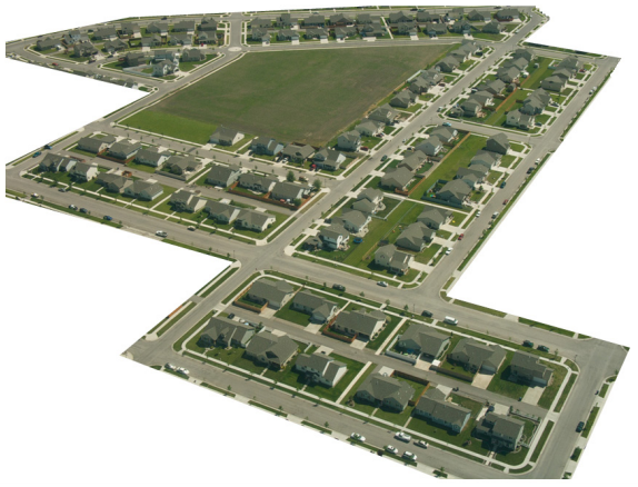
Naturally, she wants to minimize the amount of walking she has to do. Is it possible for her to walk down every street in this development without having to do any backtracking? While you might be able to answer that question just by looking at the picture for a while, it would be ideal to be able to answer the question for any picture regardless of its complexity.

To do that, we first need to simplify the picture into a form that is easier to work with. We can do that by drawing a simple line for each street. Where streets intersect, we will place a dot.

Fig2_5_2

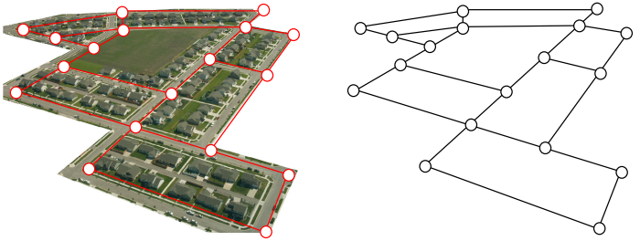
This type of simplified picture is called a graph.

Graphs, Vertices, and Edges

A graph consists of a set of dots, called vertices, and a set of edges connecting pairs of vertices.

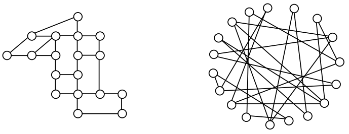
While we drew our original graph to correspond with the picture we had, there is nothing particularly important about the layout when we analyze a graph. Both of the graphs below are equivalent to the one drawn above.

Fig2_5_3

You probably already noticed that we are using the term graph differently than you may have used the term in the past to describe the graph of a mathematical function.

Watch the video below to get another perspective of drawing a street network graph.

Example

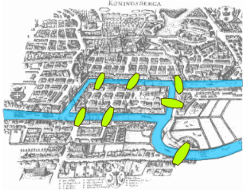Fig2_5_4 Back in the 18th century in the Prussian city of Königsberg, a river ran through the city and seven bridges crossed the forks of the river. The river and the bridges are highlighted in the picture to the right.^[1]

As a weekend amusement, townsfolk would see if they could find a route that would take them across every bridge once and return them to where they started.

In the following video we present another view of the Königsberg bridge problem.

Leonard Euler (pronounced OY-lur), one of the most prolific mathematicians ever, looked at this problem in 1735, laying the foundation for graph theory as a field in mathematics. To analyze this problem, Euler introduced edges representing the bridges:

Fig2_5_5

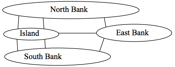
Since the size of each land mass it is not relevant to the question of bridge crossings, each can be shrunk down to a vertex representing the location:

Fig2_5_6

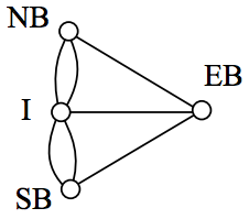
Notice that in this graph there are two edges connecting the north bank and island, corresponding to the two bridges in the original drawing. Depending upon the interpretation of edges and vertices appropriate to a scenario, it is entirely possible and reasonable to have more than one edge connecting two vertices.

While we haven’t answered the actual question yet of whether or not there is a route which crosses every bridge once and returns to the starting location, the graph provides the foundation for exploring this question.

Definitions

While we loosely defined some terminology earlier, we now will try to be more specific.

Vertex

A vertex is a dot in the graph that could represent an intersection of streets, a land mass, or a general location, like “work” or “school”. Vertices are often connected by edges. Note that vertices only occur when a dot is explicitly placed, not whenever two edges cross. Imagine a freeway overpass—the freeway and side street cross, but it is not possible to change from the side street to the freeway at that point, so there is no intersection and no vertex would be placed.

Edges

Edges connect pairs of vertices. An edge can represent a physical connection between locations, like a street, or simply that a route connecting the two locations exists, like an airline flight.

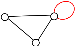
Loop

A loop is a special type of edge that connects a vertex to itself. Loops are not used much in street network graphs.

Fig2_5_7

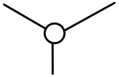
Degree of a vertex

The degree of a vertex is the number of edges meeting at that vertex. It is possible for a vertex to have a degree of zero or larger.

Degree 0	Degree 1	Degree 2	Degree 3	Degree 4

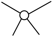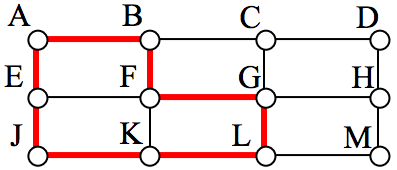
Path

A path is a sequence of vertices using the edges. Usually we are interested in a path between two vertices. For example, a path from vertex A to vertex M is shown below. It is one of many possible paths in this graph.

Fig2_5_13

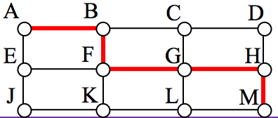
Circuit

A circuit is a path that begins and ends at the same vertex. A circuit starting and ending at vertex A is shown below.

Fig2_5_14

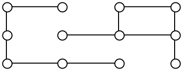
Connected

A graph is connected if there is a path from any vertex to any other vertex. Every graph drawn so far has been connected. The graph below is disconnected; there is no way to get from the vertices on the left to the vertices on the right.

Fig2_5_15

Weights

Depending upon the problem being solved, sometimes weights are assigned to the edges. The weights could represent the distance between two locations, the travel time, or the travel cost. It is important to note that the distance between vertices in a graph does not necessarily correspond to the weight of an edge.

Try It

1.The graph below shows 5 cities. The weights on the edges represent the airfare for a one -way flight between the cities.
a. How many vertices and edges does the graph have?
b. Is the graph connected?
c. What is the degree of the vertex representing LA?
d. If you fly from Seattle to Dallas to Atlanta, is that a path or a circuit?
e. If you fly from LA to Chicago to Dallas to LA, is that a path or a circuit.

Shortest Path

When you visit a website like Google Maps or use your Smartphone to ask for directions from home to your Aunt’s house in Pasadena, you are usually looking for a shortest path between the two locations. These computer applications use representations of the street maps as graphs, with estimated driving times as edge weights.

While often it is possible to find a shortest path on a small graph by guess-and-check, our goal in this chapter is to develop methods to solve complex problems in a systematic way by following algorithms. An algorithm is a step-by-step procedure for solving a problem. Dijkstra’s (pronounced dike-stra) algorithm will find the shortest path between two vertices.

Dijkstra’s Algorithm

1. Mark the ending vertex with a distance of zero. Designate this vertex as current.

2. Find all vertices leading to the current vertex. Calculate their distances to the end. Since we already know the distance the current vertex is from the end, this will just require adding the most recent edge. Don’t record this distance if it is longer than a previously recorded distance.

3. Mark the current vertex as visited. We will never look at this vertex again.

4. Mark the vertex with the smallest distance as current, and repeat from step 2.

EXAMPLE

Suppose you need to travel from Tacoma, WA (vertex T) to Yakima, WA (vertex Y). Looking at a map, it looks like driving through Auburn (A) then Mount Rainier (MR) might be shortest, but it’s not totally clear since that road is probably slower than taking the major highway through North Bend (NB). A graph with travel times in minutes is shown below. An alternate route through Eatonville (E) and Packwood (P) is also shown.

Step 1: Mark the ending vertex with a distance of zero. The distances will be recorded in [brackets] after the vertex name

Step 2: For each vertex leading to Y, we calculate the distance to the end. For example, NB is a distance of 104 from the end, and MR is 96 from the end. Remember that distances in this case refer to the travel time in minutes.

Step 3 & 4: We mark Y as visited, and mark the vertex with the smallest recorded distance as current. At this point, P will be designated current. Back to step 2.

Step 2 (#2): For each vertex leading to P (and not leading to a visited vertex) we find the distance from the end. Since E is 96 minutes from P, and we’ve already calculated P is 76 minutes from Y, we can compute that E is 96+76 = 172 minutes from Y.

Step 3 & 4 (#2): We mark P as visited, and designate the vertex with the smallest recorded distance as current: MR. Back to step 2.

Step 2 (#3): For each vertex leading to MR (and not leading to a visited vertex) we find the distance to the end. The only vertex to be considered is A, since we’ve already visited Y and P. Adding MR’s distance 96 to the length from A to MR gives the distance 96+79 = 175 minutes from A to Y.

Step 3 & 4 (#3): We mark MR as visited, and designate the vertex with smallest recorded distance as current: NB. Back to step 2.

Step 2 (#4): For each vertex leading to NB, we find the distance to the end. We know the shortest distance from NB to Y is 104 and the distance from A to NB is 36, so the distance from A to Y through NB is 104+36 = 140. Since this distance is shorter than the previously calculated distance from Y to A through MR, we replace it.

Step 3 & 4 (#4): We mark NB as visited, and designate A as current, since it now has the shortest distance.

Step 2 (#5): T is the only non-visited vertex leading to A, so we calculate the distance from T to Y through A: 20+140 = 160 minutes.

Step 3 & 4 (#5): We mark A as visited, and designate E as current.

Step 2 (#6): The only non-visited vertex leading to E is T. Calculating the distance from T to Y through E, we compute 172+57 = 229 minutes. Since this is longer than the existing marked time, we do not replace it.

Step 3 (#6): We mark E as visited. Since all vertices have been visited, we are done.

From this, we know that the shortest path from Tacoma to Yakima will take 160 minutes. Tracking which sequence of edges yielded 160 minutes, we see the shortest path is T-A-NB-Y.

Dijkstra’s algorithm is an optimal algorithm, meaning that it always produces the actual shortest path, not just a path that is pretty short, provided one exists. This algorithm is also efficient, meaning that it can be implemented in a reasonable amount of time. Dijkstra’s algorithm takes around V2 calculations, where V is the number of vertices in a graph[1]. A graph with 100 vertices would take around 10,000 calculations. While that would be a lot to do by hand, it is not a lot for computer to handle. It is because of this efficiency that your car’s GPS unit can compute driving directions in only a few seconds.

[1] It can be made to run faster through various optimizations to the implementation.

In contrast, an inefficient algorithm might try to list all possible paths then compute the length of each path. Trying to list all possible paths could easily take 1025 calculations to compute the shortest path with only 25 vertices; that’s a 1 with 25 zeros after it! To put that in perspective, the fastest computer in the world would still spend over 1000 years analyzing all those paths.

EXAMPLE

A shipping company needs to route a package from Washington, D.C. to San Diego, CA. To minimize costs, the package will first be sent to their processing center in Baltimore, MD then sent as part of mass shipments between their various processing centers, ending up in their processing center in Bakersfield, CA. From there it will be delivered in a small truck to San Diego.

The travel times, in hours, between their processing centers are shown in the table below. Three hours has been added to each travel time for processing. Find the shortest path from Baltimore to Bakersfield.

	Baltimore	Denver	Dallas	Chicago	Atlanta	Bakersfield
Baltimore	*			15	14
Denver		*		18	24	19
Dallas			*	18	15	25
Chicago	15	18	18	*	14
Atlanta	14	24	15	14	*
Bakersfield		19	25			*

While we could draw a graph, we can also work directly from the table.

Step 1: The ending vertex, Bakersfield, is marked as current.

Step 2: All cities connected to Bakersfield, in this case Denver and Dallas, have their distances calculated; we’ll mark those distances in the column headers.

Step 3 & 4: Mark Bakersfield as visited. Here, we are doing it by shading the corresponding row and column of the table. We mark Denver as current, shown in bold, since it is the vertex with the shortest distance.

	Baltimore	Denver [19]	Dallas [25]	Chicago	Atlanta	Bakersfield [0]
Baltimore	*			15	14
Denver		*		18	24	19
Dallas			*	18	15	25
Chicago	15	18	18	*	14
Atlanta	14	24	15	14	*
Bakersfield		19	25			*

Step 2 (#2): For cities connected to Denver, calculate distance to the end. For example, Chicago is 18 hours from Denver, and Denver is 19 hours from the end, the distance for Chicago to the end is 18+19 = 37 (Chicago to Denver to Bakersfield). Atlanta is 24 hours from Denver, so the distance to the end is 24+19 = 43 (Atlanta to Denver to Bakersfield).

Step 3 & 4 (#2): We mark Denver as visited and mark Dallas as current.

	Baltimore	Denver [19]	Dallas [25]	Chicago [37]	Atlanta [43]	Bakersfield [0]
Baltimore	*			15	14
Denver		*		18	24	19
Dallas			*	18	15	25
Chicago	15	18	18	*	14
Atlanta	14	24	15	14	*
Bakersfield		19	25			*

Step 2 (#3): For cities connected to Dallas, calculate the distance to the end. For Chicago, the distance from Chicago to Dallas is 18 and from Dallas to the end is 25, so the distance from Chicago to the end through Dallas would be 18+25 = 43. Since this is longer than the currently marked distance for Chicago, we do not replace it. For Atlanta, we calculate 15+25 = 40. Since this is shorter than the currently marked distance for Atlanta, we replace the existing distance.

Step 3 & 4 (#3): We mark Dallas as visited, and mark Chicago as current.

	Baltimore	Denver [19]	Dallas [25]	Chicago [37]	Atlanta [40]	Bakersfield [0]
Baltimore	*			15	14
Denver		*		18	24	19
Dallas			*	18	15	25
Chicago	15	18	18	*	14
Atlanta	14	24	15	14	*
Bakersfield		19	25			*

Step 2 (#4): Baltimore and Atlanta are the only non-visited cities connected to Chicago. For Baltimore, we calculate 15+37 = 52 and mark that distance. For Atlanta, we calculate 14+37 = 51. Since this is longer than the existing distance of 40 for Atlanta, we do not replace that distance.

Step 3 & 4 (#4): Mark Chicago as visited and Atlanta as current.

	Baltimore [52]	Denver [19]	Dallas [25]	Chicago [37]	Atlanta [40]	Bakersfield [0]
Baltimore	*			15	14
Denver		*		18	24	19
Dallas			*	18	15	25
Chicago	15	18	18	*	14
Atlanta	14	24	15	14	*
Bakersfield		19	25			*

Step 2 (#5): The distance from Atlanta to Baltimore is 14. Adding that to the distance already calculated for Atlanta gives a total distance of 14+40 = 54 hours from Baltimore to Bakersfield through Atlanta. Since this is larger than the currently calculated distance, we do not replace the distance for Baltimore.

Step 3 & 4 (#5): We mark Atlanta as visited. All cities have been visited and we are done.

The shortest route from Baltimore to Bakersfield will take 52 hours, and will route through Chicago and Denver.

TRY IT NOW

Find the shortest path between vertices A and G in the graph below.

The following video summarizes the topics covered on this page.

Bogdan Giuşcă. http://en.wikipedia.org/wiki/File:Konigsberg_bridges.png ↵

Module 4: Graph Theory

Learning Outcomes

Elements of Graph Theory

Drawing Graphs

Example

Graphs, Vertices, and Edges

Example

Definitions

Vertex

Edges

Loop

Degree of a vertex

Path

Circuit

Connected

Weights

Try It

Shortest Path

Dijkstra’s Algorithm

EXAMPLE

EXAMPLE

TRY IT NOW

Candela Citations