Learning Outcomes
- Recognize that all differentiable functions have closed-form derivative functions, but not all integrable functions have closed-form antiderivatives in terms of elementary functions
- Find upper and lower bounds for the area under a curve when the Fundamental Theorem of Calculus, Part 2, cannot be used
- Describe how bounds relate to the maximum possible error of an approximation
At this point on our calculus journey, we have developed the tools to find the derivative function of any differentiable function. Take, for example, the following function.
[latex]f(x)=\left[\ln\left(\tan^2\left(\frac{1}{x^{2}+3\sqrt{x}}\right)\right)\cos^{-1}\left(\frac{3x^{2}+5x-1}{22x+1}\right)+10x^{3^{x^{2}}}\right]^{e^{\sin(x^{3.2})}}[/latex]
If we were asked to find the derivative function of [latex]f(x)[/latex], it may take us multiple pages, but by methodically applying the Chain Rule, the Quotient Rule, the Product Rule, the Sum Rule, and the formulas for derivatives we’ve discovered so far, we could find a closed-form expression for [latex]f'(x)[/latex] (which, of course, would only be defined for [latex]x[/latex]-values in the domain of [latex]f(x)[/latex] at which the function is differentiable). By cutting some corners and letting Wolfram|Alpha find the derivative function for us, we see that it is:
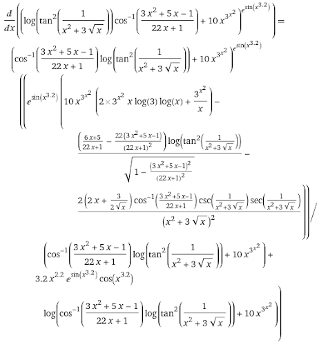
Don’t worry—we won’t be asked to do anything quite that crazy by hand. But the point is that for any differentiable function we are given, we can apply the tools in our calculus toolbelt to find the closed-form expression of its derivative function.
Integration, on the other hand, is not quite as simple. Up to this point, we’ve relied heavily on the Fundamental Theorem of calculus, Part 2, to compute definite integrals, which requires that an antiderivative of a function exists. However, there are many functions which are integrable but have no antiderivative in terms of standard elementary functions we’ve seen so far. Take, for example, the following function
[latex]g(x)=\frac{1}{\sqrt{2\pi}}e^{-\frac{1}{2}x^{2}}[/latex]
If we were asked to compute the definite integral [latex]\displaystyle\int _{0}^{1} g(x)dx[/latex], the graphical area of which is shown in the figure below, could we use the Fundamental Theorem of Calculus, Part 2? Try this on your own for a moment. Can you find an antiderivative of [latex]g(x)[/latex] in terms of elementary functions (which are the functions we learned in Module 1)?
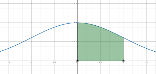
If your conclusion is “no,” then you are correct. While the function looks simple, it does not have an antiderivative in terms of elementary functions. In Calculus II we will learn some additional techniques to find antiderivatives and indefinite integrals, such as integration by parts and partial fraction decompositions, but even those cannot help us here. In fact, finding an antiderivative of [latex]g(x)[/latex] requires the introduction of special functions that are themselves defined in terms of integrals. Because of this, any antiderivative will be sufficiently complicated to the point that we could not simply apply the Fundamental Theorem of Calculus, Part 2, if we had it to find the answer. (If you’re curious, you can look up the error function [latex]\text{erf}(x)[/latex].)
What can we do, then, to find [latex]\displaystyle\int _{0}^{1} g(x)dx[/latex] if we cannot find an antiderivative of [latex]g(x)[/latex] in terms of elementary functions? The answer is that we can approximate the definite integral! Remember that in the first section of this module, before learning about indefinite and definite integrals, we first learned about using Riemann Sums to approximate the area under a curve. This method of approximating may not give us an exact answer, but it can get us mighty close to one when we’ve exhausted the tools in our calculus toolbelt. Additionally, there are some tricks to use when approximating any value in mathematics that can make an approximation extremely useful.
Let’s arbitrarily choose to use a left-endpoint Riemann Sum to approximate the definite integral [latex]\displaystyle\int _{0}^{1} g(x)dx[/latex] where [latex]g(x)[/latex] is defined as above. If we split the interval [latex][0,1][/latex] into [latex]n[/latex] subintervals of length [latex]\frac{1}{n}[/latex], then the left-endpoint Riemann sum is
[latex]L_{n}={\displaystyle\sum _{i=1}^{n}} g\left(\frac{i-1}{n}\right)\cdot\frac{1}{n}[/latex].
If we were to arbitrarily choose [latex]n=10[/latex], then our approximation would be
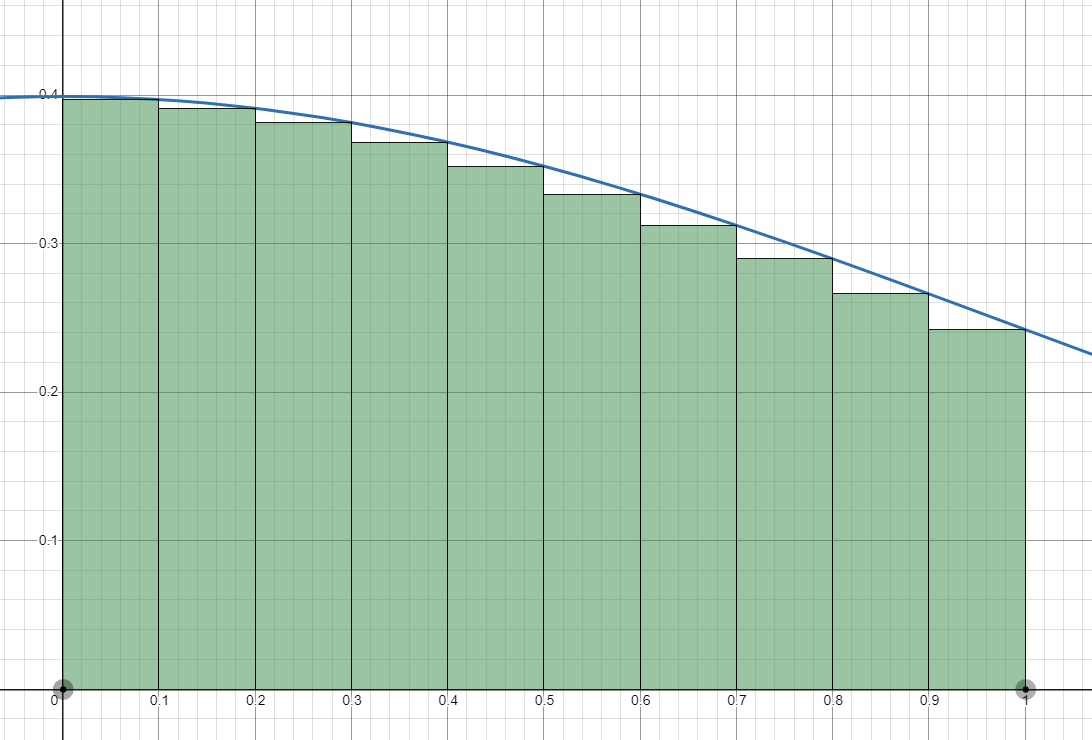
[latex]{\displaystyle\int _{0}^{1}} \frac{1}{\sqrt{2\pi}}e^{-\frac{1}{2}x^{2}}dx\approx L_{10}={\displaystyle\sum_{i=1}^{10}}\left[\frac{1}{\sqrt{2\pi}}e^{-\frac{1}{2}(i-1/10)^{2}}\cdot\frac{1}{10}\right]\approx0.349[/latex].
Graphically, this left-endpoint sum with 10 subintervals looks as follows.
Now, if we were to tell someone, “We have an approximation for [latex]\displaystyle\int _{0}^{1} g(x)dx[/latex], and it is [latex]0.349[/latex]!” how useful would that information be to them? They may counter with, “Well that’s great, but how close to the true value is your approximation? How large could your error be?” Take a moment to think about this. How could you respond to that question?
This is where the concept of using bounds for approximation comes in handy. Instead of reporting a number for an approximation of [latex]\displaystyle\int _{0}^{1} g(x)dx[/latex], if we could report an upper bound and a lower bound for the true value, that would provide much more information! With bounds, we know an interval of values that contains the true value, and if we choose a number from the interval as our approximation, we know the maximum amount of error that could be associated with the approximation.
So how do we find upper and lower bounds? Recall from the first section of this module the concept of Upper Sums and Lower Sums. An upper sum (where we use the maximum function value on each subinterval for the height of the associated rectangle) is always a weak over-approximation of the true area. Similarly, a lower sum (where we use the minimum function value on each subinterval for the height of the associate rectangle) is always a weak under-approximation of the true area (“weak” meaning that the associated inequalities are not strict). Thus, we can find an upper and lower sum and state
[latex]\text{Lower Sum}\le\text{True Value}\le\text{Upper Sum}[/latex].
In our example, [latex]g(x)=\frac{1}{\sqrt{2\pi}} e^{-\frac{1}{2}x^2}[/latex] is decreasing over the interval [latex][0,1][/latex]. Therefore, left endpoints of subintervals will correspond to maximum function values, so left-endpoint Riemann Sums will be upper sums. Similarly, right endpoints of subintervals will correspond to minimum function values, so right-endpoint Riemann sums will be lower sums.
A right-endpoint Riemann Sum to approximate [latex]\displaystyle\int _{0}^{1} g(x)dx[/latex] with [latex]n[/latex] subintervals is
[latex]R_{n}={\displaystyle\sum _{i=1}^{n}} g\left(\frac{i}{n}\right)\cdot\frac{1}{n}[/latex]
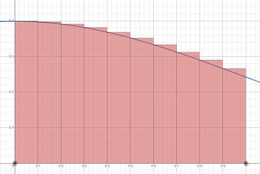
Sticking with [latex]n=10[/latex] as we chose previously, our right-endpoint approximation is
[latex]{\displaystyle\int _{0}^{1}} \frac{1}{\sqrt{2\pi}}e^{-\frac{1}{2}x^{2}}dx\approx R_{10}={\displaystyle\sum_{i=1}^{10}}\left[\frac{1}{\sqrt{2\pi}}e^{-\frac{1}{2}(i/10)^{2}}\cdot\frac{1}{10}\right]\approx0.333[/latex].
Graphically, this right-endpoint sum with [latex]10[/latex] subintervals looks as follows.
Now we have an upper sum [latex]L_{10}[/latex] and a lower sum [latex]R_{10}[/latex], meaning we can state [latex]R_{10}\le\displaystyle\int _{0}^{1} g(x)dx\le L_{10}[/latex]. Therefore,
[latex]0.333\le{\displaystyle\int _{0}^{1}} \frac{1}{\sqrt{2\pi}}e^{-\frac{1}{2}x^{2}}dx\le 0.349[/latex].
Another way to say this is that we know that the true value of [latex]{\displaystyle\int _{0}^{1}} \frac{1}{\sqrt{2\pi}}e^{-\frac{1}{2}x^{2}}dx[/latex] must lie in the interval [latex][0.333, 0.349][/latex]. If we were to choose a value from that interval to use for our approximation, what is the maximum distance that approximation could be from the true value of the definite integral? In other words, what is the largest possible error associated with that approximation?
Suppose we choose the midpoint of the interval [latex][0.333,0.349][/latex], which is [latex]\text{midpoint }=\frac{0.333+0.349}{2}=0.341[/latex], as our approximation. Since the true value we are approximating must lie in the interval [latex][0.333,0.349][/latex], the farthest our approximation could be from [latex]{\displaystyle\int _{0}^{1}} \frac{1}{\sqrt{2\pi}}e^{-\frac{1}{2}x^{2}}dx[/latex] is the distance from the midpoint to the endpoints of the interval. Let [latex]\varepsilon (x)[/latex] be the maximum error that could be associated with the approximation [latex]x[/latex]. Then,
[latex]\varepsilon(0.341)=0.349-0.341=0.341-0.333=0.008[/latex].
In words, we can say that the furthest away that our approximation [latex]0.341[/latex] could be from the true value of [latex]{\displaystyle\int _{0}^{1}} \frac{1}{\sqrt{2\pi}}e^{-\frac{1}{2}x^{2}}dx[/latex] is [latex]0.008[/latex].
Now, there is no magical reason we chose [latex]n=10[/latex] for the number of subintervals. As we choose larger and larger [latex]n[/latex], the interval for our approximation would grow smaller and smaller, as would the maximum error. Computers are able to perform these types of calculations extremely efficiently for very large [latex]n[/latex], and often have to do so when trying to compute a definite integral for a function with no antiderivative in terms of elementary functions.
Try It
Consider the function [latex]f(x)=\sqrt{1-x^{4}}[/latex]. Can you find [latex]\displaystyle\int _{-1}^{0} f(x)dx[/latex] using the Fundamental Theorem of Calculus, Part 2? If not, provide an upper bound and a lower bound for the true value of the definite integral. If you were to choose a single value from that interval to use as an approximation, what is the maximum error that could be associated with that approximation?
Candela Citations
- Approximating Integrals. Authored by: Sidney Tate. Provided by: Lumen Learning. License: CC BY: Attribution
- Calculus Volume 2. Authored by: Gilbert Strang, Edwin (Jed) Herman. Provided by: OpenStax. Located at: https://openstax.org/books/calculus-volume-2/pages/1-introduction. License: CC BY-NC-SA: Attribution-NonCommercial-ShareAlike. License Terms: Access for free at https://openstax.org/books/calculus-volume-2/pages/1-introduction
