Learning Outcomes
- Write the terms of a sequence defined by a recursive formula
- Calculate the limit of a function as 𝑥 increases or decreases without bound
- Recognize when to apply L’Hôpital’s rule
In the Sequences section, we will look at ordered lists of numbers (sequences) and determine whether they converge or diverge. Here we will review how to evaluate a recursive (recurrence) formula, take limits at infinity, and apply L’Hôpital’s Rule.
Use a Recursive Formula
A recursive formula is a formula that defines its value at a particular input using the result of the previous input(s).
A recursive formula always has two parts: the value of an initial input and an equation defining each term in terms of preceding terms. For example, suppose we know the following:
So, the first four terms are [latex]3,5,9,\text{ and},17[/latex].
How To: Given a recursive formula with only the first term provided, write the first [latex]n[/latex] terms of a sequence.
- Identify the initial term, [latex]{a}_{1}[/latex], which is given as part of the formula. This is the first term.
- To find the second term, [latex]{a}_{2}[/latex], substitute the initial term into the formula for [latex]{a}_{n - 1}[/latex]. Solve.
- To find the third term, [latex]{a}_{3}[/latex], substitute the second term into the formula. Solve.
- Repeat until you have solved for the [latex]n\text{th}[/latex] term.
Example: Writing the Terms of a Sequence Defined by a Recursive Formula
Write the first five terms of the sequence defined by the recursive formula.
[latex]\begin{align} {a}_{1}&=9 \\ {a}_{n}&=3{a}_{n - 1}-20\text{, for }n\ge 2 \end{align}[/latex]
Try It
Write the first five terms of the sequence defined by the recursive formula.
[latex]\begin{align}{a}_{1}&=2\\ {a}_{n}&=2{a}_{n - 1}+1\text{, for }n\ge 2\end{align}[/latex]
Try It
Take Limits at Infinity
Recall that [latex]\underset{x \to a}{\lim}f(x)=L[/latex] means [latex]f(x)[/latex] becomes arbitrarily close to [latex]L[/latex] as long as [latex]x[/latex] is sufficiently close to [latex]a[/latex]. We can extend this idea to limits at infinity. For example, consider the function [latex]f(x)=2+\frac{1}{x}[/latex]. As can be seen graphically in Figure 1 and numerically in the table beneath it, as the values of [latex]x[/latex] get larger, the values of [latex]f(x)[/latex] approach 2. We say the limit as [latex]x[/latex] approaches [latex]\infty[/latex] of [latex]f(x)[/latex] is 2 and write [latex]\underset{x\to \infty }{\lim}f(x)=2[/latex]. Similarly, for [latex]x<0[/latex], as the values [latex]|x|[/latex] get larger, the values of [latex]f(x)[/latex] approaches 2. We say the limit as [latex]x[/latex] approaches [latex]−\infty[/latex] of [latex]f(x)[/latex] is 2 and write [latex]\underset{x\to a}{\lim}f(x)=2[/latex].
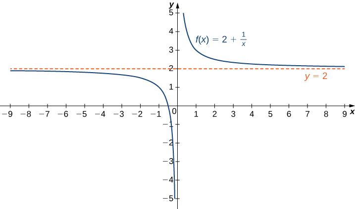
Figure 1. The function approaches the asymptote [latex]y=2[/latex] as [latex]x[/latex] approaches [latex]\pm \infty[/latex].
| [latex]x[/latex] | 10 | 100 | 1,000 | 10,000 |
| [latex]2+\frac{1}{x}[/latex] | 2.1 | 2.01 | 2.001 | 2.0001 |
| [latex]x[/latex] | -10 | -100 | -1000 | -10,000 |
| [latex]2+\frac{1}{x}[/latex] | 1.9 | 1.99 | 1.999 | 1.9999 |
More generally, for any function [latex]f[/latex], we say the limit as [latex]x \to \infty[/latex] of [latex]f(x)[/latex] is [latex]L[/latex] if [latex]f(x)[/latex] becomes arbitrarily close to [latex]L[/latex] as long as [latex]x[/latex] is sufficiently large. In that case, we write [latex]\underset{x\to \infty}{\lim}f(x)=L[/latex]. Similarly, we say the limit as [latex]x\to −\infty[/latex] of [latex]f(x)[/latex] is [latex]L[/latex] if [latex]f(x)[/latex] becomes arbitrarily close to [latex]L[/latex] as long as [latex]x<0[/latex] and [latex]|x|[/latex] is sufficiently large. In that case, we write [latex]\underset{x\to −\infty }{\lim}f(x)=L[/latex]. We now look at the definition of a function having a limit at infinity.
Definition
(Informal) If the values of [latex]f(x)[/latex] become arbitrarily close to [latex]L[/latex] as [latex]x[/latex] becomes sufficiently large, we say the function [latex]f[/latex] has a limit at infinity and write
If the values of [latex]f(x)[/latex] becomes arbitrarily close to [latex]L[/latex] for [latex]x<0[/latex] as [latex]|x|[/latex] becomes sufficiently large, we say that the function [latex]f[/latex] has a limit at negative infinity and write
If the values [latex]f(x)[/latex] are getting arbitrarily close to some finite value [latex]L[/latex] as [latex]x\to \infty[/latex] or [latex]x\to −\infty[/latex], the graph of [latex]f[/latex] approaches the line [latex]y=L[/latex]. In that case, the line [latex]y=L[/latex] is a horizontal asymptote of [latex]f[/latex] (Figure 2). For example, for the function [latex]f(x)=\frac{1}{x}[/latex], since [latex]\underset{x\to \infty }{\lim}f(x)=0[/latex], the line [latex]y=0[/latex] is a horizontal asymptote of [latex]f(x)=\frac{1}{x}[/latex].
Definition
If [latex]\underset{x\to \infty }{\lim}f(x)=L[/latex] or [latex]\underset{x \to −\infty}{\lim}f(x)=L[/latex], we say the line [latex]y=L[/latex] is a horizontal asymptote of [latex]f[/latex].
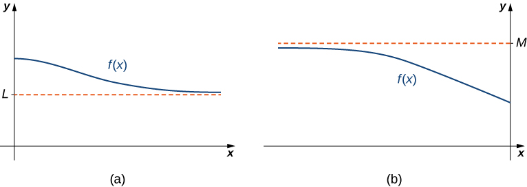
Figure 2. (a) As [latex]x\to \infty[/latex], the values of [latex]f[/latex] are getting arbitrarily close to [latex]L[/latex]. The line [latex]y=L[/latex] is a horizontal asymptote of [latex]f[/latex]. (b) As [latex]x\to −\infty[/latex], the values of [latex]f[/latex] are getting arbitrarily close to [latex]M[/latex]. The line [latex]y=M[/latex] is a horizontal asymptote of [latex]f[/latex].
A function cannot cross a vertical asymptote because the graph must approach infinity (or negative infinity) from at least one direction as [latex]x[/latex] approaches the vertical asymptote. However, a function may cross a horizontal asymptote. In fact, a function may cross a horizontal asymptote an unlimited number of times. For example, the function [latex]f(x)=\frac{ \cos x}{x}+1[/latex] shown in Figure 3 intersects the horizontal asymptote [latex]y=1[/latex] an infinite number of times as it oscillates around the asymptote with ever-decreasing amplitude.
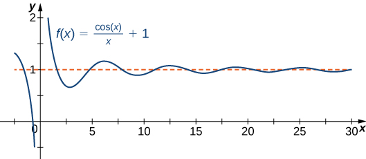
Figure 3. The graph of [latex]f(x)=\cos x/x+1[/latex] crosses its horizontal asymptote [latex]y=1[/latex] an infinite number of times.
Example: Computing Limits at Infinity
For each of the following functions [latex]f[/latex], evaluate [latex]\underset{x\to \infty }{\lim}f(x)[/latex] and [latex]\underset{x\to −\infty }{\lim}f(x)[/latex].
- [latex]f(x)=5-\frac{2}{x^2}[/latex]
- [latex]f(x)=\dfrac{\sin x}{x}[/latex]
- [latex]f(x)= \tan^{-1} (x)[/latex]
Try It
Evaluate [latex]\underset{x\to −\infty}{\lim}\left(3+\frac{4}{x}\right)[/latex] and [latex]\underset{x\to \infty }{\lim}\left(3+\frac{4}{x}\right)[/latex]. Determine the horizontal asymptotes of [latex]f(x)=3+\frac{4}{x}[/latex], if any.
Infinite Limits at Infinity
Sometimes the values of a function [latex]f[/latex] become arbitrarily large as [latex]x\to \infty[/latex] (or as [latex]x\to −\infty )[/latex]. In this case, we write [latex]\underset{x\to \infty }{\lim}f(x)=\infty[/latex] (or [latex]\underset{x\to −\infty }{\lim}f(x)=\infty )[/latex]. On the other hand, if the values of [latex]f[/latex] are negative but become arbitrarily large in magnitude as [latex]x\to \infty[/latex] (or as [latex]x\to −\infty )[/latex], we write [latex]\underset{x\to \infty }{\lim}f(x)=−\infty[/latex] (or [latex]\underset{x\to −\infty }{\lim}f(x)=−\infty )[/latex].
For example, consider the function [latex]f(x)=x^3[/latex]. As seen in the table below and Figure 2, as [latex]x\to \infty[/latex] the values [latex]f(x)[/latex] become arbitrarily large. Therefore, [latex]\underset{x\to \infty }{\lim}x^3=\infty[/latex]. On the other hand, as [latex]x\to −\infty[/latex], the values of [latex]f(x)=x^3[/latex] are negative but become arbitrarily large in magnitude. Consequently, [latex]\underset{x\to −\infty }{\lim}x^3=−\infty[/latex].
| [latex]x[/latex] | 10 | 20 | 50 | 100 | 1000 |
| [latex]x^3[/latex] | 1000 | 8000 | 125,000 | 1,000,000 | 1,000,000,000 |
| [latex]x[/latex] | -10 | -20 | -50 | -100 | -1000 |
| [latex]x^3[/latex] | -1000 | -8000 | -125,000 | -1,000,000 | -1,000,000,000 |
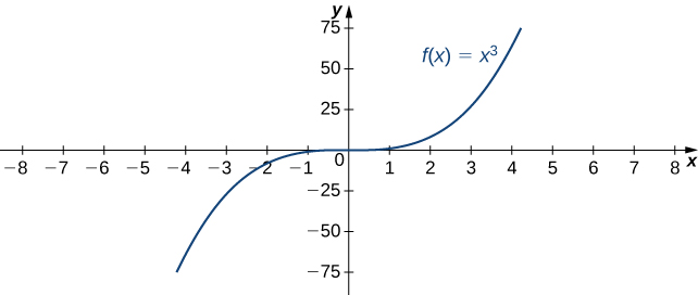
Figure 2. For this function, the functional values approach infinity as [latex]x\to \pm \infty[/latex].
Definition
(Informal) We say a function [latex]f[/latex] has an infinite limit at infinity and write
if [latex]f(x)[/latex] becomes arbitrarily large for [latex]x[/latex] sufficiently large. We say a function has a negative infinite limit at infinity and write
if [latex]f(x)<0[/latex] and [latex]|f(x)|[/latex] becomes arbitrarily large for [latex]x[/latex] sufficiently large. Similarly, we can define infinite limits as [latex]x\to −\infty[/latex].
Try It
Find [latex]\underset{x\to \infty }{\lim}3x^2[/latex].
Try It
Apply L’Hôpital’s Rule
L’Hôpital’s rule can be used to evaluate limits involving the quotient of two functions. Consider
If [latex]\underset{x\to a}{\lim}f(x)=L_1[/latex] and [latex]\underset{x\to a}{\lim}g(x)=L_2 \ne 0[/latex], then
However, what happens if [latex]\underset{x\to a}{\lim}f(x)=0[/latex] and [latex]\underset{x\to a}{\lim}g(x)=0[/latex]? We call this one of the indeterminate forms, of type [latex]\frac{0}{0}[/latex]. This is considered an indeterminate form because we cannot determine the exact behavior of [latex]\frac{f(x)}{g(x)}[/latex] as [latex]x\to a[/latex] without further analysis. We have seen examples of this earlier in the text. For example, consider
For the first of these examples, we can evaluate the limit by factoring the numerator and writing
For [latex]\underset{x\to 0}{\lim}\frac{\sin x}{x}[/latex] we were able to show, using a geometric argument, that
Here we use a different technique for evaluating limits such as these. Not only does this technique provide an easier way to evaluate these limits, but also, and more important, it provides us with a way to evaluate many other limits that we could not calculate previously.
The idea behind L’Hôpital’s rule can be explained using local linear approximations. Consider two differentiable functions [latex]f[/latex] and [latex]g[/latex] such that [latex]\underset{x\to a}{\lim}f(x)=0=\underset{x\to a}{\lim}g(x)[/latex] and such that [latex]g^{\prime}(a)\ne 0[/latex] For [latex]x[/latex] near [latex]a[/latex], we can write
and
Therefore,
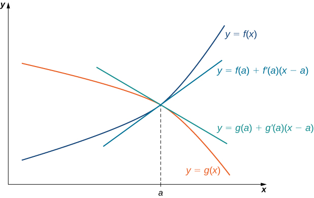
Figure 1. If [latex]\underset{x\to a}{\lim}f(x)=\underset{x\to a}{\lim}g(x)[/latex], then the ratio [latex]f(x)/g(x)[/latex] is approximately equal to the ratio of their linear approximations near [latex]a[/latex].
Since [latex]f[/latex] is differentiable at [latex]a[/latex], then [latex]f[/latex] is continuous at [latex]a[/latex], and therefore [latex]f(a)=\underset{x\to a}{\lim}f(x)=0[/latex]. Similarly, [latex]g(a)=\underset{x\to a}{\lim}g(x)=0[/latex]. If we also assume that [latex]f^{\prime}[/latex] and [latex]g^{\prime}[/latex] are continuous at [latex]x=a[/latex], then [latex]f^{\prime}(a)=\underset{x\to a}{\lim}f^{\prime}(x)[/latex] and [latex]g^{\prime}(a)=\underset{x\to a}{\lim}g^{\prime}(x)[/latex]. Using these ideas, we conclude that
Note that the assumption that [latex]f^{\prime}[/latex] and [latex]g^{\prime}[/latex] are continuous at [latex]a[/latex] and [latex]g^{\prime}(a)\ne 0[/latex] can be loosened. We state L’Hôpital’s rule formally for the indeterminate form [latex]\frac{0}{0}[/latex]. Also note that the notation [latex]\frac{0}{0}[/latex] does not mean we are actually dividing zero by zero. Rather, we are using the notation [latex]\frac{0}{0}[/latex] to represent a quotient of limits, each of which is zero.
L’Hôpital’s Rule (0/0 Case)
Suppose [latex]f[/latex] and [latex]g[/latex] are differentiable functions over an open interval containing [latex]a[/latex], except possibly at [latex]a[/latex]. If [latex]\underset{x\to a}{\lim}f(x)=0[/latex] and [latex]\underset{x\to a}{\lim}g(x)=0[/latex], then
assuming the limit on the right exists or is [latex]\infty[/latex] or [latex]−\infty[/latex]. This result also holds if we are considering one-sided limits, or if [latex]a=\infty[/latex] or [latex]-\infty[/latex].
Example: Applying L’Hôpital’s Rule (0/0 Case)
Evaluate each of the following limits by applying L’Hôpital’s rule.
- [latex]\underset{x\to 0}{\lim}\dfrac{1- \cos x}{x}[/latex]
- [latex]\underset{x\to 1}{\lim}\dfrac{\sin (\pi x)}{\ln x}[/latex]
- [latex]\underset{x\to \infty }{\lim}\dfrac{e^{\frac{1}{x}}-1}{\frac{1}{x}}[/latex]
- [latex]\underset{x\to 0}{\lim}\dfrac{\sin x-x}{x^2}[/latex]
Try It
Evaluate [latex]\underset{x\to 0}{\lim}\dfrac{x}{\tan x}[/latex].
We can also use L’Hôpital’s rule to evaluate limits of quotients [latex]\frac{f(x)}{g(x)}[/latex] in which [latex]f(x)\to \pm \infty[/latex] and [latex]g(x)\to \pm \infty[/latex]. Limits of this form are classified as indeterminate forms of type [latex]\infty / \infty[/latex]. Again, note that we are not actually dividing [latex]\infty[/latex] by [latex]\infty[/latex]. Since [latex]\infty[/latex] is not a real number, that is impossible; rather, [latex]\infty / \infty[/latex] is used to represent a quotient of limits, each of which is [latex]\infty[/latex] or [latex]−\infty[/latex].
L’Hôpital’s Rule ([latex]\infty / \infty[/latex] Case)
Suppose [latex]f[/latex] and [latex]g[/latex] are differentiable functions over an open interval containing [latex]a[/latex], except possibly at [latex]a[/latex]. Suppose [latex]\underset{x\to a}{\lim}f(x)=\infty[/latex] (or [latex]−\infty[/latex]) and [latex]\underset{x\to a}{\lim}g(x)=\infty[/latex] (or [latex]−\infty[/latex]). Then,
assuming the limit on the right exists or is [latex]\infty[/latex] or [latex]−\infty[/latex]. This result also holds if the limit is infinite, if [latex]a=\infty[/latex] or [latex]−\infty[/latex], or the limit is one-sided.
Example: Applying L’Hôpital’s Rule ([latex]\infty /\infty[/latex] Case)
Evaluate each of the following limits by applying L’Hôpital’s rule.
- [latex]\underset{x\to \infty }{\lim}\dfrac{3x+5}{2x+1}[/latex]
- [latex]\underset{x\to 0^+}{\lim}\dfrac{\ln x}{\cot x}[/latex]
Try It
Evaluate [latex]\underset{x\to \infty }{\lim}\dfrac{\ln x}{5x}[/latex]
Candela Citations
- Modification and Revision. Provided by: Lumen Learning. License: CC BY: Attribution
- College Algebra Corequisite. Provided by: Lumen Learning. Located at: https://courses.lumenlearning.com/waymakercollegealgebracorequisite/. License: CC BY: Attribution
- Precalculus. Provided by: Lumen Learning. Located at: https://courses.lumenlearning.com/precalculus/. License: CC BY: Attribution
