In the following exercises, find the Taylor polynomials of degree two approximating the given function centered at the given point.
1. [latex]f\left(x\right)=1+x+{x}^{2}[/latex] at [latex]a=1[/latex]
2. [latex]f\left(x\right)=1+x+{x}^{2}[/latex] at [latex]a=-1[/latex]
Show Solution
[latex]f\left(-1\right)=1;{f}^{\prime }\left(-1\right)=-1;f\text{''}\left(-1\right)=2;f\left(x\right)=1-\left(x+1\right)+{\left(x+1\right)}^{2}[/latex]
3. [latex]f\left(x\right)=\cos\left(2x\right)[/latex] at [latex]a=\pi[/latex]
4. [latex]f\left(x\right)=\sin\left(2x\right)[/latex] at [latex]a=\frac{\pi }{2}[/latex]
Show Solution
[latex]{f}^{\prime }\left(x\right)=2\cos\left(2x\right);f\text{''}\left(x\right)=-4\sin\left(2x\right);{p}_{2}\left(x\right)=-2\left(x-\frac{\pi }{2}\right)[/latex]
5. [latex]f\left(x\right)=\sqrt{x}[/latex] at [latex]a=4[/latex]
6. [latex]f\left(x\right)=\text{ln}x[/latex] at [latex]a=1[/latex]
Show Solution
[latex]{f}^{\prime }\left(x\right)=\frac{1}{x};f\text{''}\left(x\right)=-\frac{1}{{x}^{2}};{p}_{2}\left(x\right)=0+\left(x - 1\right)-\frac{1}{2}{\left(x - 1\right)}^{2}[/latex]
7. [latex]f\left(x\right)=\frac{1}{x}[/latex] at [latex]a=1[/latex]
8. [latex]f\left(x\right)={e}^{x}[/latex] at [latex]a=1[/latex]
Show Solution
[latex]{p}_{2}\left(x\right)=e+e\left(x - 1\right)+\frac{e}{2}{\left(x - 1\right)}^{2}[/latex]
In the following exercises, verify that the given choice of n in the remainder estimate [latex]|{R}_{n}|\le \frac{M}{\left(n+1\right)\text{!}}{\left(x-a\right)}^{n+1}[/latex], where M is the maximum value of [latex]|{f}^{\left(n+1\right)}\left(z\right)|[/latex] on the interval between a and the indicated point, yields [latex]|{R}_{n}|\le \frac{1}{1000}[/latex]. Find the value of the Taylor polynomial pn of [latex]f[/latex] at the indicated point.
9. [T] [latex]\sqrt{10};a=9,n=3[/latex]
10. [T] [latex]{\left(28\right)}^{\frac{1}{3}};a=27,n=1[/latex]
Show Solution
[latex]\frac{{d}^{2}}{d{x}^{2}}{x}^{\frac{1}{3}}=-\frac{2}{9{x}^{\frac{5}{3}}}\ge -0.00092\ldots[/latex] when [latex]x\ge 28[/latex] so the remainder estimate applies to the linear approximation [latex]{x}^{\frac{1}{3}}\approx {p}_{1}\left(27\right)=3+\frac{x - 27}{27}[/latex], which gives [latex]{\left(28\right)}^{\frac{1}{3}}\approx 3+\frac{1}{27}=3.\overline{037}[/latex], while [latex]{\left(28\right)}^{\frac{1}{3}}\approx 3.03658[/latex].
11. [T] [latex]\sin\left(6\right);a=2\pi ,n=5[/latex]
12. [T] e2; [latex]a=0,n=9[/latex]
Show Solution
Using the estimate [latex]\frac{{2}^{10}}{10\text{!}}<0.000283[/latex] we can use the Taylor expansion of order 9 to estimate [latex]e^{x}[/latex] at [latex]x=2[/latex]. as [latex]{e}^{2}\approx {p}_{9}\left(2\right)=1+2+\frac{{2}^{2}}{2}+\frac{{2}^{3}}{6}+\cdots+\frac{{2}^{9}}{9\text{!}}=7.3887\ldots[/latex] whereas [latex]{e}^{2}\approx 7.3891[/latex].
13. [T] [latex]\cos\left(\frac{\pi }{5}\right);a=0,n=4[/latex]
14. [T] [latex]\text{ln}\left(2\right);a=1,n=1000[/latex]
Show Solution
Since [latex]\frac{{d}^{n}}{d{x}^{n}}\left(\text{ln}x\right)={\left(-1\right)}^{n - 1}\frac{\left(n - 1\right)\text{!}}{{x}^{n}},{R}_{1000}\approx \frac{1}{1001}[/latex]. One has [latex]{p}_{1000}\left(1\right)=\displaystyle\sum _{n=1}^{1000}\frac{{\left(-1\right)}^{n - 1}}{n}\approx 0.6936[/latex] whereas [latex]\text{ln}\left(2\right)\approx 0.6931\cdots[/latex].
15. Integrate the approximation [latex]\sin{t}\approx t-\frac{{t}^{3}}{6}+\frac{{t}^{5}}{120}-\frac{{t}^{7}}{5040}[/latex] evaluated at πt to approximate [latex]{\displaystyle\int }_{0}^{1}\frac{\sin\pi t}{\pi t}dt[/latex].
16. Integrate the approximation [latex]{e}^{x}\approx 1+x+\frac{{x}^{2}}{2}+\cdots+\frac{{x}^{6}}{720}[/latex] evaluated at −x2 to approximate [latex]{\displaystyle\int }_{0}^{1}{e}^{\text{-}{x}^{2}}dx[/latex].
Show Solution
[latex]{\displaystyle\int }_{0}^{1}\left(1-{x}^{2}+\frac{{x}^{4}}{2}-\frac{{x}^{6}}{6}+\frac{{x}^{8}}{24}-\frac{{x}^{10}}{120}+\frac{{x}^{12}}{720}\right)dx[/latex]
[latex]=1-\frac{{1}^{3}}{3}+\frac{{1}^{5}}{10}-\frac{{1}^{7}}{42}+\frac{{1}^{9}}{9\cdot 24}-\frac{{1}^{11}}{120\cdot 11}+\frac{{1}^{13}}{720\cdot 13}\approx 0.74683[/latex] whereas [latex]{\displaystyle\int }_{0}^{1}{e}^{\text{-}{x}^{2}}dx\approx 0.74682[/latex].
In the following exercises, find the smallest value of n such that the remainder estimate [latex]|{R}_{n}|\le \frac{M}{\left(n+1\right)\text{!}}{\left(x-a\right)}^{n+1}[/latex], where M is the maximum value of [latex]|{f}^{\left(n+1\right)}\left(z\right)|[/latex] on the interval between a and the indicated point, yields [latex]|{R}_{n}|\le \frac{1}{1000}[/latex] on the indicated interval.
17. [latex]f\left(x\right)=\sin{x}[/latex] on [latex]\left[\text{-}\pi ,\pi \right],a=0[/latex]
18. [latex]f\left(x\right)=\cos{x}[/latex] on [latex]\left[-\frac{\pi }{2},\frac{\pi }{2}\right],a=0[/latex]
Show Solution
Since [latex]{f}^{\left(n+1\right)}\left(z\right)[/latex] is [latex]\sin{z}[/latex] or [latex]\cos{z}[/latex], we have [latex]M=1[/latex]. Since [latex]|x - 0|\le \frac{\pi }{2}[/latex], we seek the smallest n such that [latex]\frac{{\pi }^{n+1}}{{2}^{n+1}\left(n+1\right)\text{!}}\le 0.001[/latex]. The smallest such value is [latex]n=7[/latex]. The remainder estimate is [latex]{R}_{7}\le 0.00092[/latex].
19. [latex]f\left(x\right)={e}^{-2x}[/latex] on [latex]\left[-1,1\right],a=0[/latex]
20. [latex]f\left(x\right)={e}^{\text{-}x}[/latex] on [latex]\left[-3,3\right],a=0[/latex]
Show Solution
Since [latex]{f}^{\left(n+1\right)}\left(z\right)=\pm{e}^{\text{-}z}[/latex] one has [latex]M={e}^{3}[/latex]. Since [latex]|x - 0|\le 3[/latex], one seeks the smallest n such that [latex]\frac{{3}^{n+1}{e}^{3}}{\left(n+1\right)\text{!}}\le 0.001[/latex]. The smallest such value is [latex]n=14[/latex]. The remainder estimate is [latex]{R}_{14}\le 0.000220[/latex].
In the following exercises, the maximum of the right-hand side of the remainder estimate [latex]|{R}_{1}|\le \frac{\text{max}|f\text{''}\left(z\right)|}{2}{R}^{2}[/latex] on [latex]\left[a-R,a+R\right][/latex] occurs at a or [latex]a\pm R[/latex]. Estimate the maximum value of R such that [latex]\frac{\text{max}|f\text{''}\left(z\right)|}{2}{R}^{2}\le 0.1[/latex] on [latex]\left[a-R,a+R\right][/latex] by plotting this maximum as a function of R.
21. [T] ex approximated by [latex]1+x,a=0[/latex]
22. [T] [latex]\sin{x}[/latex] approximated by x, [latex]a=0[/latex]
Show Solution
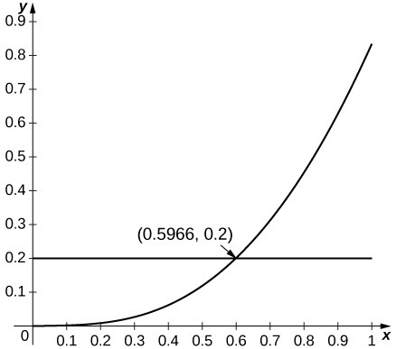
Since [latex]\sin{x}[/latex] is increasing for small x and since [latex]\mathrm{si}n\text{''}x=\text{-}\sin{x}[/latex], the estimate applies whenever [latex]{R}^{2}\sin\left(R\right)\le 0.2[/latex], which applies up to [latex]R=0.596[/latex].
23. [T] [latex]\text{ln}x[/latex] approximated by [latex]x - 1,a=1[/latex]
24. [T] [latex]\cos{x}[/latex] approximated by [latex]1,a=0[/latex]
Show Solution
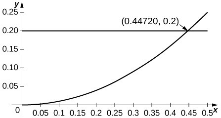
Since the second derivative of [latex]\cos{x}[/latex] is [latex]\text{-}\cos{x}[/latex] and since [latex]\cos{x}[/latex] is decreasing away from [latex]x=0[/latex], the estimate applies when [latex]{R}^{2}\cos{R}\le 0.2[/latex] or [latex]R\le 0.447[/latex].
In the following exercises, find the Taylor series of the given function centered at the indicated point.
25. [latex]{x}^{4}[/latex] at [latex]a=-1[/latex]
26. [latex]1+x+{x}^{2}+{x}^{3}[/latex] at [latex]a=-1[/latex]
Show Solution
[latex]{\left(x+1\right)}^{3}-2{\left(x+1\right)}^{2}+2\left(x+1\right)[/latex]
27. [latex]\sin{x}[/latex] at [latex]a=\pi[/latex]
28. [latex]\cos{x}[/latex] at [latex]a=2\pi[/latex]
Show Solution
Values of derivatives are the same as for [latex]x=0[/latex] so [latex]\cos{x}={\displaystyle\sum _{n=0}^{\infty }\left(-1\right)}^{n}\frac{{\left(x - 2\pi \right)}^{2n}}{\left(2n\right)\text{!}}[/latex]
29. [latex]\sin{x}[/latex] at [latex]x=\frac{\pi }{2}[/latex]
30. [latex]\cos{x}[/latex] at [latex]x=\frac{\pi }{2}[/latex]
Show Solution
[latex]\cos\left(\frac{\pi }{2}\right)=0,\text{-}\sin\left(\frac{\pi }{2}\right)=-1[/latex] so [latex]\cos{x}=\displaystyle\sum _{n=0}^{\infty }{\left(-1\right)}^{n+1}\frac{{\left(x-\frac{\pi }{2}\right)}^{2n+1}}{\left(2n+1\right)\text{!}}[/latex], which is also [latex]\text{-}\cos\left(x-\frac{\pi }{2}\right)[/latex].
31. [latex]{e}^{x}[/latex] at [latex]a=-1[/latex]
32. [latex]{e}^{x}[/latex] at [latex]a=1[/latex]
Show Solution
The derivatives are [latex]{f}^{\left(n\right)}\left(1\right)=e[/latex] so [latex]{e}^{x}=e\displaystyle\sum _{n=0}^{\infty }\frac{{\left(x - 1\right)}^{n}}{n\text{!}}[/latex].
33. [latex]\frac{1}{{\left(x - 1\right)}^{2}}[/latex] at [latex]a=0[/latex] (Hint: Differentiate [latex]\frac{1}{1-x}.[/latex])
34. [latex]\frac{1}{{\left(x - 1\right)}^{3}}[/latex] at [latex]a=0[/latex]
Show Solution
[latex]\frac{1}{{\left(x - 1\right)}^{3}}=\text{-}\left(\frac{1}{2}\right)\frac{{d}^{2}}{d{x}^{2}}\frac{1}{1-x}=\text{-}\displaystyle\sum _{n=0}^{\infty }\left(\frac{\left(n+2\right)\left(n+1\right){x}^{n}}{2}\right)[/latex]
35. [latex]F\left(x\right)={\displaystyle\int }_{0}^{x}\cos\left(\sqrt{t}\right)dt;f\left(t\right)=\displaystyle\sum _{n=0}^{\infty }{\left(-1\right)}^{n}\frac{{t}^{n}}{\left(2n\right)\text{!}}[/latex] at [latex]a=0[/latex] (Note: [latex]f[/latex] is the Taylor series of [latex]\cos\left(\sqrt{t}\right).[/latex])
In the following exercises, compute the Taylor series of each function around [latex]x=1[/latex].
36. [latex]f\left(x\right)=2-x[/latex]
Show Solution
[latex]2-x=1-\left(x - 1\right)[/latex]
37. [latex]f\left(x\right)={x}^{3}[/latex]
38. [latex]f\left(x\right)={\left(x - 2\right)}^{2}[/latex]
Show Solution
[latex]{\left(\left(x - 1\right)-1\right)}^{2}={\left(x - 1\right)}^{2}-2\left(x - 1\right)+1[/latex]
39. [latex]f\left(x\right)=\text{ln}x[/latex]
40. [latex]f\left(x\right)=\frac{1}{x}[/latex]
Show Solution
[latex]\frac{1}{1-\left(1-x\right)}=\displaystyle\sum _{n=0}^{\infty }{\left(-1\right)}^{n}{\left(x - 1\right)}^{n}[/latex]
41. [latex]f\left(x\right)=\frac{1}{2x-{x}^{2}}[/latex]
42. [latex]f\left(x\right)=\frac{x}{4x - 2{x}^{2}-1}[/latex]
Show Solution
[latex]x\displaystyle\sum _{n=0}^{\infty }{2}^{n}{\left(1-x\right)}^{2n}=\displaystyle\sum _{n=0}^{\infty }{2}^{n}{\left(x - 1\right)}^{2n+1}+\displaystyle\sum _{n=0}^{\infty }{2}^{n}{\left(x - 1\right)}^{2n}[/latex]
43. [latex]f\left(x\right)={e}^{\text{-}x}[/latex]
44. [latex]f\left(x\right)={e}^{2x}[/latex]
Show Solution
[latex]{e}^{2x}={e}^{2\left(x - 1\right)+2}={e}^{2}\displaystyle\sum _{n=0}^{\infty }\frac{{2}^{n}{\left(x - 1\right)}^{n}}{n\text{!}}[/latex]
[T] In the following exercises, identify the value of x such that the given series [latex]\displaystyle\sum _{n=0}^{\infty }{a}_{n}[/latex] is the value of the Maclaurin series of [latex]f\left(x\right)[/latex] at [latex]x[/latex]. Approximate the value of [latex]f\left(x\right)[/latex] using [latex]{S}_{10}=\displaystyle\sum _{n=0}^{10}{a}_{n}[/latex].
45. [latex]\displaystyle\sum _{n=0}^{\infty }\frac{1}{n\text{!}}[/latex]
46. [latex]\displaystyle\sum _{n=0}^{\infty }\frac{{2}^{n}}{n\text{!}}[/latex]
Show Solution
[latex]x={e}^{2};{S}_{10}=\frac{34,913}{4725}\approx 7.3889947[/latex]
47. [latex]\displaystyle\sum _{n=0}^{\infty }\frac{{\left(-1\right)}^{n}{\left(2\pi \right)}^{2n}}{\left(2n\right)\text{!}}[/latex]
48. [latex]\displaystyle\sum _{n=0}^{\infty }\frac{{\left(-1\right)}^{n}{\left(2\pi \right)}^{2n+1}}{\left(2n+1\right)\text{!}}[/latex]
Show Solution
[latex]\sin\left(2\pi \right)=0;{S}_{10}=8.27\times {10}^{-5}[/latex]
The following exercises make use of the functions [latex]{S}_{5}\left(x\right)=x-\frac{{x}^{3}}{6}+\frac{{x}^{5}}{120}[/latex] and [latex]{C}_{4}\left(x\right)=1-\frac{{x}^{2}}{2}+\frac{{x}^{4}}{24}[/latex] on [latex]\left[\text{-}\pi ,\pi \right][/latex].
49. [T] Plot [latex]{\sin}^{2}x-{\left({S}_{5}\left(x\right)\right)}^{2}[/latex] on [latex]\left[\text{-}\pi ,\pi \right][/latex]. Compare the maximum difference with the square of the Taylor remainder estimate for [latex]\sin{x}[/latex].
50. [T] Plot [latex]{\cos}^{2}x-{\left({C}_{4}\left(x\right)\right)}^{2}[/latex] on [latex]\left[\text{-}\pi ,\pi \right][/latex]. Compare the maximum difference with the square of the Taylor remainder estimate for [latex]\cos{x}[/latex].
Show Solution
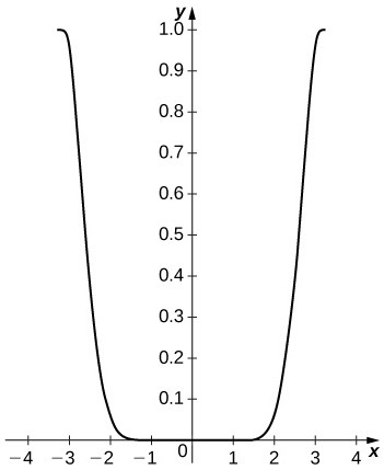
The difference is small on the interior of the interval but approaches [latex]1[/latex] near the endpoints. The remainder estimate is [latex]|{R}_{4}|=\frac{{\pi }^{5}}{120}\approx 2.552[/latex].
51. [T] Plot [latex]|2{S}_{5}\left(x\right){C}_{4}\left(x\right)-\sin\left(2x\right)|[/latex] on [latex]\left[\text{-}\pi ,\pi \right][/latex].
52. [T] Compare [latex]\frac{{S}_{5}\left(x\right)}{{C}_{4}\left(x\right)}[/latex] on [latex]\left[-1,1\right][/latex] to [latex]\tan{x}[/latex]. Compare this with the Taylor remainder estimate for the approximation of [latex]\tan{x}[/latex] by [latex]x+\frac{{x}^{3}}{3}+\frac{2{x}^{5}}{15}[/latex].
Show Solution
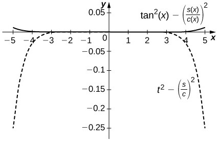
The difference is on the order of [latex]{10}^{-4}[/latex] on [latex]\left[-1,1\right][/latex] while the Taylor approximation error is around [latex]0.1[/latex] near [latex]\pm 1[/latex]. The top curve is a plot of [latex]{\tan}^{2}x-{\left(\frac{{S}_{5}\left(x\right)}{{C}_{4}\left(x\right)}\right)}^{2}[/latex] and the lower dashed plot shows [latex]{t}^{2}-{\left(\frac{{S}_{5}}{{C}_{4}}\right)}^{2}[/latex].
53. [T] Plot [latex]{e}^{x}-{e}_{4}\left(x\right)[/latex] where [latex]{e}_{4}\left(x\right)=1+x+\frac{{x}^{2}}{2}+\frac{{x}^{3}}{6}+\frac{{x}^{4}}{24}[/latex] on [latex]\left[0,2\right][/latex]. Compare the maximum error with the Taylor remainder estimate.
54. (Taylor approximations and root finding.) Recall that Newton’s method [latex]{x}_{n+1}={x}_{n}-\frac{f\left({x}_{n}\right)}{f\prime \left({x}_{n}\right)}[/latex] approximates solutions of [latex]f\left(x\right)=0[/latex] near the input [latex]{x}_{0}[/latex].
- If [latex]f[/latex] and [latex]g[/latex] are inverse functions, explain why a solution of [latex]g\left(x\right)=a[/latex] is the value [latex]f\left(a\right)\text{of}f[/latex].
- Let [latex]{p}_{N}\left(x\right)[/latex] be the [latex]N\text{th}[/latex] degree Maclaurin polynomial of [latex]{e}^{x}[/latex]. Use Newton’s method to approximate solutions of [latex]{p}_{N}\left(x\right)-2=0[/latex] for [latex]N=4,5,6[/latex].
- Explain why the approximate roots of [latex]{p}_{N}\left(x\right)-2=0[/latex] are approximate values of [latex]\text{ln}\left(2\right)[/latex].
Show Solution
a. Answers will vary. b. The following are the [latex]{x}_{n}[/latex] values after [latex]10[/latex] iterations of Newton’s method to approximation a root of [latex]{p}_{N}\left(x\right)-2=0\text{:}[/latex] for [latex]N=4,x=0.6939...[/latex]; for [latex]N=5,x=0.6932...[/latex]; for [latex]N=6,x=0.69315...[/latex];. (Note: [latex]\text{ln}\left(2\right)=0.69314...[/latex]) c. Answers will vary.
In the following exercises, use the fact that if [latex]q\left(x\right)=\displaystyle\sum _{n=1}^{\infty }{a}_{n}{\left(x-c\right)}^{n}[/latex] converges in an interval containing [latex]c[/latex], then [latex]\underset{x\to c}{\text{lim}}q\left(x\right)={a}_{0}^{}[/latex] to evaluate each limit using Taylor series.
55. [latex]\underset{x\to 0}{\text{lim}}\frac{\cos{x} - 1}{{x}^{2}}[/latex]
56. [latex]\underset{x\to 0}{\text{lim}}\frac{\text{ln}\left(1-{x}^{2}\right)}{{x}^{2}}[/latex]
Show Solution
[latex]\frac{\text{ln}\left(1-{x}^{2}\right)}{{x}^{2}}\to \text{-}1[/latex]
57. [latex]\underset{x\to 0}{\text{lim}}\frac{{e}^{{x}^{2}}-{x}^{2}-1}{{x}^{4}}[/latex]
58. [latex]\underset{x\to {0}^{+}}{\text{lim}}\frac{\cos\left(\sqrt{x}\right)-1}{2x}[/latex]
Show Solution
[latex]\frac{\cos\left(\sqrt{x}\right)-1}{2x}\approx \frac{\left(1-\frac{x}{2}+\frac{{x}^{2}}{4\text{!}}-\cdots\right)-1}{2x}\to -\frac{1}{4}[/latex]
Candela Citations
CC licensed content, Shared previously
