Learning Outcomes
- Find the general antiderivative of a given function
- Evaluate trigonometric functions at specific angle measures
- Use the Fundamental Theorem of Calculus, Part 2, to evaluate definite integrals
- Solve rational equations by clearing denominators
- Solve for a variable in a square root equation
- Convert between radical and exponent notations
- Solve for a variable in a complex radical or rational exponent equation
- Calculate the limit of a function as 𝑥 increases or decreases without bound
In the sections that discuss double and triple integrals, we will learn how to integrate functions with more than one independent variable over various types of regions in various coordinate systems. Here we will review basic integration techniques, evaluating trigonometric functions, evaluating definite integrals using the Second Fundamental Theorem of Calculus, manipulating equations, and how to find limits at infinity.
Indefinite Integrals
Definition
Given a function [latex]f[/latex], the indefinite integral of [latex]f[/latex], denoted
is the most general antiderivative of [latex]f[/latex]. If [latex]F[/latex] is an antiderivative of [latex]f[/latex], then
The expression [latex]f(x)[/latex] is called the integrand and the variable [latex]x[/latex] is the variable of integration.
Power Rule for Integrals
For [latex]n \ne −1[/latex],
Evaluating indefinite integrals for some other functions is also a straightforward calculation. The following table lists the indefinite integrals for several common functions. A more complete list appears in Appendix B: Table of Derivatives.
| Differentiation Formula | Indefinite Integral |
|---|---|
| [latex]\frac{d}{dx}(k)=0[/latex] | [latex]\displaystyle\int kdx=\displaystyle\int kx^0 dx=kx+C[/latex] |
| [latex]\frac{d}{dx}(x^n)=nx^{n-1}[/latex] | [latex]\displaystyle\int x^n dx=\frac{x^{n+1}}{n+1}+C[/latex] for [latex]n\ne −1[/latex] |
| [latex]\frac{d}{dx}(\ln |x|)=\frac{1}{x}[/latex] | [latex]\displaystyle\int \frac{1}{x}dx=\ln |x|+C[/latex] |
| [latex]\frac{d}{dx}(e^x)=e^x[/latex] | [latex]\displaystyle\int e^x dx=e^x+C[/latex] |
| [latex]\frac{d}{dx}(\sin x)= \cos x[/latex] | [latex]\displaystyle\int \cos x dx= \sin x+C[/latex] |
| [latex]\frac{d}{dx}(\cos x)=− \sin x[/latex] | [latex]\displaystyle\int \sin x dx=− \cos x+C[/latex] |
| [latex]\frac{d}{dx}(\tan x)= \sec^2 x[/latex] | [latex]\displaystyle\int \sec^2 x dx= \tan x+C[/latex] |
| [latex]\frac{d}{dx}(\csc x)=−\csc x \cot x[/latex] | [latex]\displaystyle\int \csc x \cot x dx=−\csc x+C[/latex] |
| [latex]\frac{d}{dx}(\sec x)= \sec x \tan x[/latex] | [latex]\displaystyle\int \sec x \tan x dx= \sec x+C[/latex] |
| [latex]\frac{d}{dx}(\cot x)=−\csc^2 x[/latex] | [latex]\displaystyle\int \csc^2 x dx=−\cot x+C[/latex] |
| [latex]\frac{d}{dx}( \sin^{-1} x)=\frac{1}{\sqrt{1-x^2}}[/latex] | [latex]\displaystyle\int \frac{1}{\sqrt{1-x^2}} dx= \sin^{-1} x+C[/latex] |
| [latex]\frac{d}{dx}(\tan^{-1} x)=\frac{1}{1+x^2}[/latex] | [latex]\displaystyle\int \frac{1}{1+x^2} dx= \tan^{-1} x+C[/latex] |
| [latex]\frac{d}{dx}(\sec^{-1} |x|)=\frac{1}{x\sqrt{x^2-1}}[/latex] | [latex]\displaystyle\int \frac{1}{x\sqrt{x^2-1}} dx= \sec^{-1} |x|+C[/latex] |
Properties of Indefinite Integrals
Let [latex]F[/latex] and [latex]G[/latex] be antiderivatives of [latex]f[/latex] and [latex]g[/latex], respectively, and let [latex]k[/latex] be any real number.
Sums and Differences
Constant Multiples
Example: Evaluating Indefinite Integrals
Evaluate each of the following indefinite integrals:
- [latex]\displaystyle\int (5x^3-7x^2+3x+4) dx[/latex]
- [latex]\displaystyle\int \frac{x^2+4\sqrt[3]{x}}{x} dx[/latex]
- [latex]\displaystyle\int \frac{4}{1+x^2} dx[/latex]
- [latex]\displaystyle\int \tan x \cos x dx[/latex]
Try It
Evaluate [latex]\displaystyle\int (4x^3-5x^2+x-7) dx[/latex]
Try It
Evaluate Trigonometric Functions
(also in Module 1, Skills Review for Polar Coordinates)
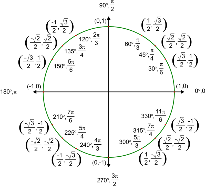
The unit circle tells us the value of cosine and sine at any of the given angle measures seen below. The first coordinate in each ordered pair is the value of cosine at the given angle measure, while the second coordinate in each ordered pair is the value of sine at the given angle measure. You will learn that all trigonometric functions can be written in terms of sine and cosine. Thus, if you can evaluate sine and cosine at various angle values, you can also evaluate the other trigonometric functions at various angle values. Take time to learn the [latex]\left(x,y\right)[/latex] coordinates of all of the major angles in the first quadrant of the unit circle.
Remember, every angle in quadrant two, three, or four has a reference angle that lies in quadrant one. The quadrant of the original angle only affects the sign (positive or negative) of a trigonometric function’s value at a given angle.
A General Note: Evaluating Tangent, Secant, Cosecant, and Cotangent Functions
If [latex]\theta[/latex] is an angle measure, then, using the unit circle,
[latex]\begin{gathered}\tan \theta=\frac{sin \theta}{cos \theta}\\ \sec \theta=\frac{1}{cos \theta}\\ \csc t=\frac{1}{sin \theta}\\ \cot \theta=\frac{cos \theta}{sin \theta}\end{gathered}[/latex]
Example: Using the Unit Circle to Find the Value of Trigonometric Functions
Find [latex]\sin \theta,\cos \theta,\tan \theta,\sec \theta,\csc \theta[/latex], and [latex]\cot \theta[/latex] when [latex]\theta=\frac{\pi }{3}[/latex].
Try It
Below are the values of all six trigonometric functions evaluated at common angle measures from Quadrant I.
| Angle | [latex]0[/latex] | [latex]\frac{\pi }{6},\text{ or }{30}^{\circ}[/latex] | [latex]\frac{\pi }{4},\text{ or } {45}^{\circ }[/latex] | [latex]\frac{\pi }{3},\text{ or }{60}^{\circ }[/latex] | [latex]\frac{\pi }{2},\text{ or }{90}^{\circ }[/latex] |
| Cosine | 1 | [latex]\frac{\sqrt{3}}{2}[/latex] | [latex]\frac{\sqrt{2}}{2}[/latex] | [latex]\frac{1}{2}[/latex] | 0 |
| Sine | 0 | [latex]\frac{1}{2}[/latex] | [latex]\frac{\sqrt{2}}{2}[/latex] | [latex]\frac{\sqrt{3}}{2}[/latex] | 1 |
| Tangent | 0 | [latex]\frac{\sqrt{3}}{3}[/latex] | 1 | [latex]\sqrt{3}[/latex] | Undefined |
| Secant | 1 | [latex]\frac{2\sqrt{3}}{3}[/latex] | [latex]\sqrt{2}[/latex] | 2 | Undefined |
| Cosecant | Undefined | 2 | [latex]\sqrt{2}[/latex] | [latex]\frac{2\sqrt{3}}{3}[/latex] | 1 |
| Cotangent | Undefined | [latex]\sqrt{3}[/latex] | 1 | [latex]\frac{\sqrt{3}}{3}[/latex] | 0 |
Fundamental Theorem of Calculus, Part 2: The Evaluation Theorem
(also in Module 3, Skills Review for Arc Length and Curvature)
The Fundamental Theorem of Calculus, Part 2 (also known as the evaluation theorem) states that if we can find an antiderivative for the integrand, then we can evaluate the definite integral by evaluating the antiderivative at the endpoints of the interval and subtracting.
The Fundamental Theorem of Calculus, Part 2
If [latex]f[/latex] is continuous over the interval [latex]\left[a,b\right][/latex] and [latex]F(x)[/latex] is any antiderivative of [latex]f(x),[/latex] then
Example: Evaluating an Integral with the Fundamental Theorem of Calculus
Use the second part of the Fundamental Theorem of Calculus to evaluate
Example: Evaluating a Definite Integral Using the Fundamental Theorem of Calculus, Part 2
Evaluate the following integral using the Fundamental Theorem of Calculus, Part 2:
[latex]{\displaystyle\int }_{1}^{9}\dfrac{x-1}{\sqrt{x}}dx.[/latex]
Try It
Use the second part of the Fundamental Theorem of Calculus to evaluate [latex]{\displaystyle\int }_{1}^{2}{x}^{-4}dx.[/latex]
Try It
Manipulate Equations
It will sometimes be necessary to change the bounds of an integral which will even require manipulating the given equation.
Manipulate Rational Equations
Equations that contain rational expressions are called rational equations. For example, [latex]\frac{2y+1}{4}=\frac{x}{3}[/latex] is a rational equation (of two variables).
One of the most straightforward ways to solve a rational equation for the indicated variable is to eliminate denominators with the common denominator and then use properties of equality to isolate the indicated variable.
Solve for [latex]y[/latex] in the equation [latex]\frac{1}{2}y-3=2-\frac{3}{4}x[/latex] by clearing the fractions in the equation first.
Multiply both sides of the equation by [latex]4[/latex], the common denominator of the fractional coefficients.
[latex]\begin{array}{c}\frac{1}{2}y-3=2-\frac{3}{4}x\\ 4\left(\frac{1}{2}y-3\right)=4\left(2-\frac{3}{4}x\right)\\\text{}\,\,\,\,4\left(\frac{1}{2}y\right)-4\left(3\right)=4\left(2\right)+4\left(-\frac{3}{4}x\right)\\2y-12=8-3x\\\underline{+12}\,\,\,\,\,\,\underline{+12}\\ 2y=20-3x\\ \frac{2y}{2}=\frac{20-3x}{2} \\ y=10-\frac{3}{2}x\end{array}[/latex]
Example: Solving a Rational Equation For a Specific Variable
Solve the equation [latex]\frac{x+5}{8}=\frac{7}{y}[/latex] for [latex]y[/latex].
In the next example, we show how to solve a rational equation with a binomial in the denominator of one term. We will use the common denominator to eliminate the denominators from both fractions. Note that the LCD is the product of both denominators because they do not share any common factors.
Example: Solving a Rational Equation For a Specific Variable
Solve the equation [latex]x=\frac{4}{3y+1}[/latex] for [latex]y[/latex].
Manipulate Radical Equations
Radical equations are equations that contain variables in the radicand (the expression under a radical symbol), such as
Radical equations are manipulated by eliminating each radical, one at a time until you have solved for the indicated variable.
A General Note: Radical Equations
An equation containing terms with a variable in the radicand is called a radical equation.
How To: Given a radical equation, solve it
- Isolate the radical expression containing your variable of interest on one side of the equal sign. Put all remaining terms on the other side.
- If the radical is a square root, then square both sides of the equation. If it is a cube root, then raise both sides of the equation to the third power. In other words, for an nth root radical, raise both sides to the nth power. Doing so eliminates the radical symbol.
- Solve the resulting equation for the variable of interest.
- If a radical term still remains, repeat steps 1–2.
Example: Solving an Equation with One Radical
Solve [latex]\sqrt{15 - 2y}=x[/latex] for [latex]y[/latex].
Try It
Solve the radical equation [latex]\sqrt{y+3}=3x - 1[/latex] for [latex]y[/latex].
Rational exponents are exponents that are fractions, where the numerator is a power and the denominator is a root. For example, [latex]{16}^{\frac{1}{2}}[/latex] is another way of writing [latex]\sqrt{16}[/latex] and [latex]{8}^{\frac{2}{3}}[/latex] is another way of writing [latex]\left(\sqrt[3]{8}\right)^2[/latex].
We can solve equations in which a variable is raised to a rational exponent by raising both sides of the equation to the reciprocal of the exponent. The reason we raise the equation to the reciprocal of the exponent is because we want to eliminate the exponent on the variable term, and a number multiplied by its reciprocal equals 1. For example, [latex]\frac{2}{3}\left(\frac{3}{2}\right)=1[/latex].
A General Note: Rational Exponents
A rational exponent indicates a power in the numerator and a root in the denominator. There are multiple ways of writing an expression, a variable, or a number with a rational exponent:
Take Limits at Infinity
Recall that [latex]\underset{x \to a}{\lim}f(x)=L[/latex] means [latex]f(x)[/latex] becomes arbitrarily close to [latex]L[/latex] as long as [latex]x[/latex] is sufficiently close to [latex]a[/latex]. We can extend this idea to limits at infinity. For example, consider the function [latex]f(x)=2+\frac{1}{x}[/latex]. As can be seen graphically below, as the values of [latex]x[/latex] get larger, the values of [latex]f(x)[/latex] approach 2. We say the limit as [latex]x[/latex] approaches [latex]\infty[/latex] of [latex]f(x)[/latex] is 2 and write [latex]\underset{x\to \infty }{\lim}f(x)=2[/latex]. Similarly, for [latex]x<0[/latex], as the values [latex]|x|[/latex] get larger, the values of [latex]f(x)[/latex] approaches 2. We say the limit as [latex]x[/latex] approaches [latex]−\infty[/latex] of [latex]f(x)[/latex] is 2 and write [latex]\underset{x\to a}{\lim}f(x)=2[/latex].
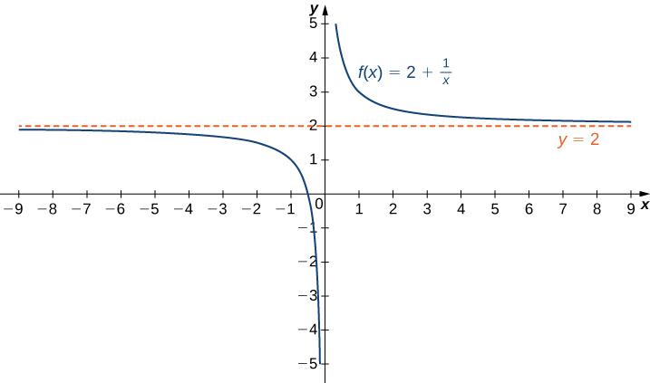
The function approaches the asymptote [latex]y=2[/latex] as [latex]x[/latex] approaches [latex]\pm \infty[/latex].
More generally, for any function [latex]f[/latex], we say the limit as [latex]x \to \infty[/latex] of [latex]f(x)[/latex] is [latex]L[/latex] if [latex]f(x)[/latex] becomes arbitrarily close to [latex]L[/latex] as long as [latex]x[/latex] is sufficiently large. In that case, we write [latex]\underset{x\to \infty}{\lim}f(x)=L[/latex]. Similarly, we say the limit as [latex]x\to −\infty[/latex] of [latex]f(x)[/latex] is [latex]L[/latex] if [latex]f(x)[/latex] becomes arbitrarily close to [latex]L[/latex] as long as [latex]x<0[/latex] and [latex]|x|[/latex] is sufficiently large. In that case, we write [latex]\underset{x\to −\infty }{\lim}f(x)=L[/latex]. We now look at the definition of a function having a limit at infinity.
Definition
(Informal) If the values of [latex]f(x)[/latex] become arbitrarily close to [latex]L[/latex] as [latex]x[/latex] becomes sufficiently large, we say the function [latex]f[/latex] has a limit at infinity and write
If the values of [latex]f(x)[/latex] becomes arbitrarily close to [latex]L[/latex] for [latex]x<0[/latex] as [latex]|x|[/latex] becomes sufficiently large, we say that the function [latex]f[/latex] has a limit at negative infinity and write
If the values [latex]f(x)[/latex] are getting arbitrarily close to some finite value [latex]L[/latex] as [latex]x\to \infty[/latex] or [latex]x\to −\infty[/latex], the graph of [latex]f[/latex] approaches the line [latex]y=L[/latex]. In that case, the line [latex]y=L[/latex] is a horizontal asymptote of [latex]f[/latex] (Figure 2). For example, for the function [latex]f(x)=\frac{1}{x}[/latex], since [latex]\underset{x\to \infty }{\lim}f(x)=0[/latex], the line [latex]y=0[/latex] is a horizontal asymptote of [latex]f(x)=\frac{1}{x}[/latex].
Definition
If [latex]\underset{x\to \infty }{\lim}f(x)=L[/latex] or [latex]\underset{x \to −\infty}{\lim}f(x)=L[/latex], we say the line [latex]y=L[/latex] is a horizontal asymptote of [latex]f[/latex].
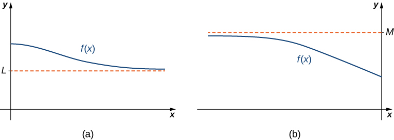
Figure 2. (a) As [latex]x\to \infty[/latex], the values of [latex]f[/latex] are getting arbitrarily close to [latex]L[/latex]. The line [latex]y=L[/latex] is a horizontal asymptote of [latex]f[/latex]. (b) As [latex]x\to −\infty[/latex], the values of [latex]f[/latex] are getting arbitrarily close to [latex]M[/latex]. The line [latex]y=M[/latex] is a horizontal asymptote of [latex]f[/latex].
A function cannot cross a vertical asymptote because the graph must approach infinity (or negative infinity) from at least one direction as [latex]x[/latex] approaches the vertical asymptote. However, a function may cross a horizontal asymptote. In fact, a function may cross a horizontal asymptote an unlimited number of times. For example, the function [latex]f(x)=\frac{ \cos x}{x}+1[/latex] shown in Figure 3 intersects the horizontal asymptote [latex]y=1[/latex] an infinite number of times as it oscillates around the asymptote with ever-decreasing amplitude.
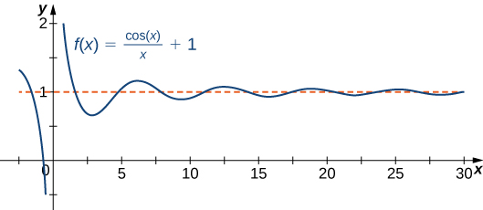
Figure 3. The graph of [latex]f(x)=\cos x/x+1[/latex] crosses its horizontal asymptote [latex]y=1[/latex] an infinite number of times.
Example: Computing Limits at Infinity
For each of the following functions [latex]f[/latex], evaluate [latex]\underset{x\to \infty }{\lim}f(x)[/latex] and [latex]\underset{x\to −\infty }{\lim}f(x)[/latex].
- [latex]f(x)=5-\frac{2}{x^2}[/latex]
- [latex]f(x)=\dfrac{\sin x}{x}[/latex]
Try It
Evaluate [latex]\underset{x\to −\infty}{\lim}\left(3+\frac{4}{x}\right)[/latex] and [latex]\underset{x\to \infty }{\lim}\left(3+\frac{4}{x}\right)[/latex].
Infinite Limits at Infinity
Sometimes the values of a function [latex]f[/latex] become arbitrarily large as [latex]x\to \infty[/latex] (or as [latex]x\to −\infty )[/latex]. In this case, we write [latex]\underset{x\to \infty }{\lim}f(x)=\infty[/latex] (or [latex]\underset{x\to −\infty }{\lim}f(x)=\infty )[/latex]. On the other hand, if the values of [latex]f[/latex] are negative but become arbitrarily large in magnitude as [latex]x\to \infty[/latex] (or as [latex]x\to −\infty )[/latex], we write [latex]\underset{x\to \infty }{\lim}f(x)=−\infty[/latex] (or [latex]\underset{x\to −\infty }{\lim}f(x)=−\infty )[/latex].
For example, consider the function [latex]f(x)=x^3[/latex]. The [latex]\underset{x\to \infty }{\lim}x^3=\infty[/latex]. On the other hand, as [latex]x\to −\infty[/latex], the values of [latex]f(x)=x^3[/latex] are negative but become arbitrarily large in magnitude. Consequently, [latex]\underset{x\to −\infty }{\lim}x^3=−\infty[/latex].
| [latex]x[/latex] | 10 | 20 | 50 | 100 | 1000 |
| [latex]x^3[/latex] | 1000 | 8000 | 125,000 | 1,000,000 | 1,000,000,000 |
| [latex]x[/latex] | -10 | -20 | -50 | -100 | -1000 |
| [latex]x^3[/latex] | -1000 | -8000 | -125,000 | -1,000,000 | -1,000,000,000 |
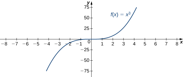
For this function, the functional values approach infinity as [latex]x\to \pm \infty[/latex].
Definition
(Informal) We say a function [latex]f[/latex] has an infinite limit at infinity and write
if [latex]f(x)[/latex] becomes arbitrarily large for [latex]x[/latex] sufficiently large. We say a function has a negative infinite limit at infinity and write
if [latex]f(x)<0[/latex] and [latex]|f(x)|[/latex] becomes arbitrarily large for [latex]x[/latex] sufficiently large. Similarly, we can define infinite limits as [latex]x\to −\infty[/latex].
Try It
Find [latex]\underset{x\to \infty }{\lim}3x^2[/latex].
Try It
Candela Citations
- Calculus Volume 1. Provided by: Lumen Learning. Located at: https://courses.lumenlearning.com/calculus1/. License: CC BY: Attribution
- Calculus Volume 2. Provided by: Lumen Learning. Located at: https://courses.lumenlearning.com/calculus2/. License: CC BY: Attribution
