Learning Objectives
By the end of this section, you will be able to:
- Explain the difference between average velocity and instantaneous velocity.
- Describe the difference between velocity and speed.
- Calculate the instantaneous velocity given the mathematical equation for the velocity.
- Calculate the speed given the instantaneous velocity.
We have now seen how to calculate the average velocity between two positions. However, since objects in the real world move continuously through space and time, we would like to find the velocity of an object at any single point. We can find the velocity of the object anywhere along its path by using some fundamental principles of calculus. This section gives us better insight into the physics of motion and will be useful in later chapters.
Instantaneous Velocity
The quantity that tells us how fast an object is moving anywhere along its path is the instantaneous velocity, usually called simply velocity. It is the average velocity between two points on the path in the limit that the time (and therefore the displacement) between the two points approaches zero. To illustrate this idea mathematically, we need to express position x as a continuous function of t denoted by x(t). The expression for the average velocity between two points using this notation is $$ \overset{\text{–}}{v}=\frac{x({t}_{2})-x({t}_{1})}{{t}_{2}-{t}_{1}}$$. To find the instantaneous velocity at any position, we let $$ {t}_{1}=t $$ and $$ {t}_{2}=t+\text{Δ}t$$. After inserting these expressions into the equation for the average velocity and taking the limit as $$ \text{Δ}t\to 0$$, we find the expression for the instantaneous velocity:
The instantaneous velocity of an object is the limit of the average velocity as the elapsed time approaches zero, or the derivative of x with respect to t:
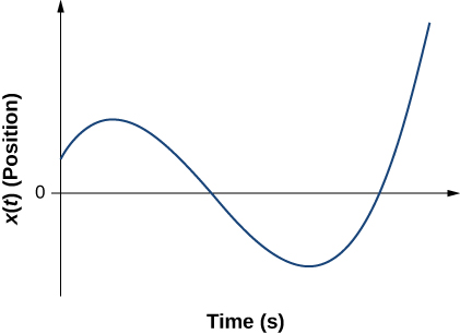
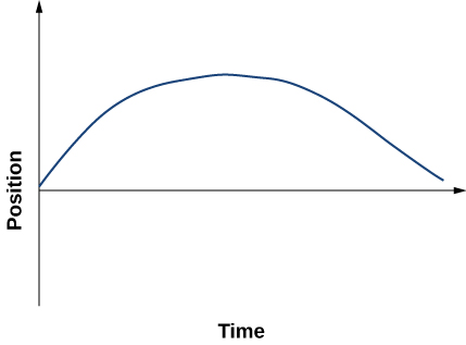
Like average velocity, instantaneous velocity is a vector with dimension of length per time. The instantaneous velocity at a specific time point $$ {t}_{0} $$ is the rate of change of the position function, which is the slope of the position function $$ x(t) $$ at $$ {t}_{0}$$. (Figure) shows how the average velocity $$ \overset{\text{–}}{v}=\frac{\text{Δ}x}{\text{Δ}t} $$ between two times approaches the instantaneous velocity at $$ {t}_{0}. $$ The instantaneous velocity is shown at time $$ {t}_{0}$$, which happens to be at the maximum of the position function. The slope of the position graph is zero at this point, and thus the instantaneous velocity is zero. At other times, $$ {t}_{1},{t}_{2}$$, and so on, the instantaneous velocity is not zero because the slope of the position graph would be positive or negative. If the position function had a minimum, the slope of the position graph would also be zero, giving an instantaneous velocity of zero there as well. Thus, the zeros of the velocity function give the minimum and maximum of the position function.
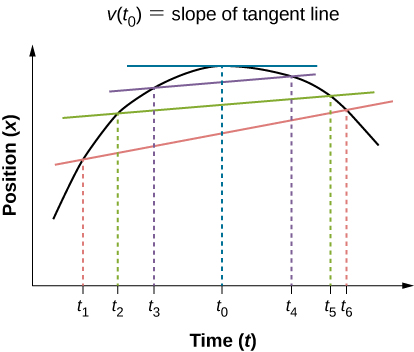
Figure 3.6 In a graph of position versus time, the instantaneous velocity is the slope of the tangent line at a given point. The average velocities $$ \overset{\text{–}}{v}=\frac{\text{Δ}x}{\text{Δ}t}=\frac{{x}_{\text{f}}-{x}_{\text{i}}}{{t}_{\text{f}}-{t}_{\text{i}}} $$ between times $$ \text{Δ}t={t}_{6}-{t}_{1},\text{Δ}t={t}_{5}-{t}_{2},\text{and}\,\text{Δ}t={t}_{4}-{t}_{3} $$ are shown. When $$ \text{Δ}t\to 0$$, the average velocity approaches the instantaneous velocity at $$ t={t}_{0}$$.
Example
Finding Velocity from a Position-Versus-Time Graph
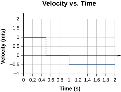
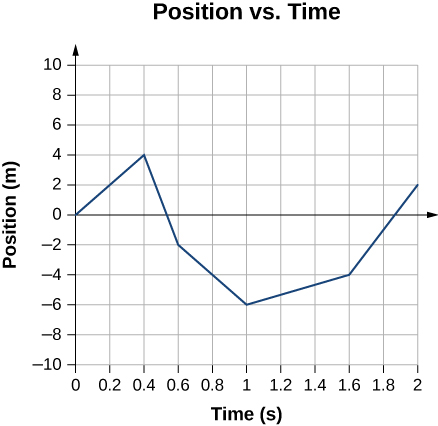
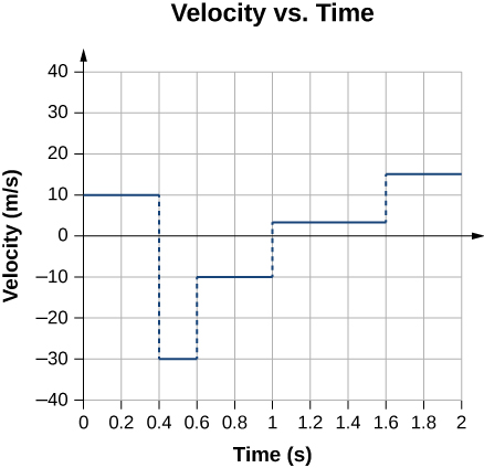
Given the position-versus-time graph of (Figure), find the velocity-versus-time graph.
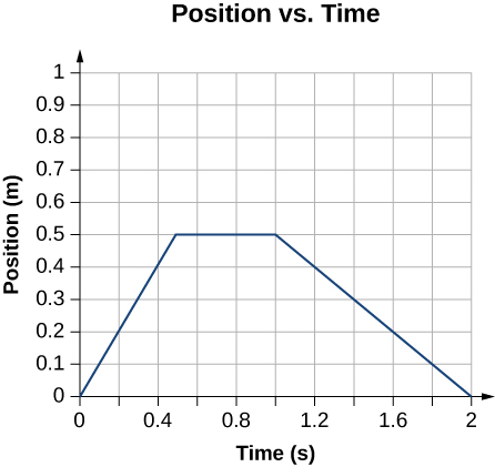
Figure 3.7 The object starts out in the positive direction, stops for a short time, and then reverses direction, heading back toward the origin. Notice that the object comes to rest instantaneously, which would require an infinite force. Thus, the graph is an approximation of motion in the real world. (The concept of force is discussed in Newton’s Laws of Motion.)
Strategy
The graph contains three straight lines during three time intervals. We find the velocity during each time interval by taking the slope of the line using the grid.
Solution
Significance
During the time interval between 0 s and 0.5 s, the object’s position is moving away from the origin and the position-versus-time curve has a positive slope. At any point along the curve during this time interval, we can find the instantaneous velocity by taking its slope, which is +1 m/s, as shown in (Figure). In the subsequent time interval, between 0.5 s and 1.0 s, the position doesn’t change and we see the slope is zero. From 1.0 s to 2.0 s, the object is moving back toward the origin and the slope is −0.5 m/s. The object has reversed direction and has a negative velocity.
Speed
In everyday language, most people use the terms speed and velocity interchangeably. In physics, however, they do not have the same meaning and are distinct concepts. One major difference is that speed has no direction; that is, speed is a scalar.
We can calculate the average speed by finding the total distance traveled divided by the elapsed time:
Average speed is not necessarily the same as the magnitude of the average velocity, which is found by dividing the magnitude of the total displacement by the elapsed time. For example, if a trip starts and ends at the same location, the total displacement is zero, and therefore the average velocity is zero. The average speed, however, is not zero, because the total distance traveled is greater than zero. If we take a road trip of 300 km and need to be at our destination at a certain time, then we would be interested in our average speed.
However, we can calculate the instantaneous speed from the magnitude of the instantaneous velocity:
If a particle is moving along the x-axis at +7.0 m/s and another particle is moving along the same axis at −7.0 m/s, they have different velocities, but both have the same speed of 7.0 m/s. Some typical speeds are shown in the following table.
| Speed | m/s | mi/h |
|---|---|---|
| Continental drift | $${10}^{-7}$$ | $$2\,×\,{10}^{-7}$$ |
| Brisk walk | 1.7 | 3.9 |
| Cyclist | 4.4 | 10 |
| Sprint runner | 12.2 | 27 |
| Rural speed limit | 24.6 | 56 |
| Official land speed record | 341.1 | 763 |
| Speed of sound at sea level | 343 | 768 |
| Space shuttle on reentry | 7800 | 17,500 |
| Escape velocity of Earth* | 11,200 | 25,000 |
| Orbital speed of Earth around the Sun | 29,783 | 66,623 |
| Speed of light in a vacuum | 299,792,458 | 670,616,629 |
Calculating Instantaneous Velocity
When calculating instantaneous velocity, we need to specify the explicit form of the position function x(t). For the moment, let’s use polynomials $$ x(t)=A{t}^{n}$$, because they are easily differentiated using the power rule of calculus:
The following example illustrates the use of (Figure).
Example
Instantaneous Velocity Versus Average Velocity
The position of a particle is given by $$ x(t)=3.0t+0.5{t}^{3}\,\text{m}$$.
- Using (Figure) and (Figure), find the instantaneous velocity at $$ t=2.0 $$ s.
- Calculate the average velocity between 1.0 s and 3.0 s.
Strategy(Figure) gives the instantaneous velocity of the particle as the derivative of the position function. Looking at the form of the position function given, we see that it is a polynomial in t. Therefore, we can use (Figure), the power rule from calculus, to find the solution. We use (Figure) to calculate the average velocity of the particle.
Solution
- $$v(t)=\frac{dx(t)}{dt}=3.0+1.5{t}^{2}\,\text{m/s}$$.Substituting t = 2.0 s into this equation gives $$ v(2.0\,\text{s})=[3.0+1.5{(2.0)}^{2}]\,\text{m/s}=9.0\,\text{m/s}$$.
- To determine the average velocity of the particle between 1.0 s and 3.0 s, we calculate the values of x(1.0 s) and x(3.0 s):
$$x(1.0\,\text{s})=[(3.0)(1.0)+0.5{(1.0)}^{3}]\,\text{m}=3.5\,\text{m}$$$$x(3.0\,\text{s})=[(3.0)(3.0)+0.5{(3.0)}^{3}]\,\text{m}=22.5\,\text{m.}$$
Then the average velocity is
$$\overset{\text{–}}{v}=\frac{x(3.0\,\text{s})-x(1.0\,\text{s})}{t(3.0\,\text{s})-t(1.0\,\text{s})}=\frac{22.5-3.5\,\text{m}}{3.0-1.0\,\text{s}}=9.5\,\text{m/s}\text{.}$$
Significance
In the limit that the time interval used to calculate $$ \overset{\text{−}}{v} $$ goes to zero, the value obtained for $$ \overset{\text{−}}{v} $$ converges to the value of v.
Example
Instantaneous Velocity Versus Speed
Consider the motion of a particle in which the position is $$ x(t)=3.0t-3{t}^{2}\,\text{m}$$.
- What is the instantaneous velocity at t = 0.25 s, t = 0.50 s, and t = 1.0 s?
- What is the speed of the particle at these times?
Strategy
The instantaneous velocity is the derivative of the position function and the speed is the magnitude of the instantaneous velocity. We use (Figure) and (Figure) to solve for instantaneous velocity.
Solution
-
Show Answer
-
Show Answer
-
Show Answer
Significance
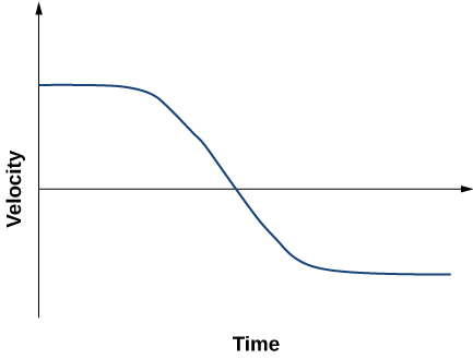
The velocity of the particle gives us direction information, indicating the particle is moving to the left (west) or right (east). The speed gives the magnitude of the velocity. By graphing the position, velocity, and speed as functions of time, we can understand these concepts visually (Figure). In (a), the graph shows the particle moving in the positive direction until t = 0.5 s, when it reverses direction. The reversal of direction can also be seen in (b) at 0.5 s where the velocity is zero and then turns negative. At 1.0 s it is back at the origin where it started. The particle’s velocity at 1.0 s in (b) is negative, because it is traveling in the negative direction. But in (c), however, its speed is positive and remains positive throughout the travel time. We can also interpret velocity as the slope of the position-versus-time graph. The slope of x(t) is decreasing toward zero, becoming zero at 0.5 s and increasingly negative thereafter. This analysis of comparing the graphs of position, velocity, and speed helps catch errors in calculations. The graphs must be consistent with each other and help interpret the calculations.
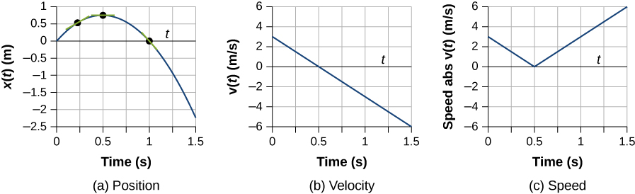
Figure 3.9 (a) Position: x(t) versus time. (b) Velocity: v(t) versus time. The slope of the position graph is the velocity. A rough comparison of the slopes of the tangent lines in (a) at 0.25 s, 0.5 s, and 1.0 s with the values for velocity at the corresponding times indicates they are the same values. (c) Speed: $$ |v(t)| $$ versus time. Speed is always a positive number.
Check Your Understanding
The position of an object as a function of time is $$ x(t)=-3{t}^{2}\,\text{m}$$. (a) What is the velocity of the object as a function of time? (b) Is the velocity ever positive? (c) What are the velocity and speed at t = 1.0 s?
Summary
- Instantaneous velocity is a continuous function of time and gives the velocity at any point in time during a particle’s motion. We can calculate the instantaneous velocity at a specific time by taking the derivative of the position function, which gives us the functional form of instantaneous velocity v(t).
- Instantaneous velocity is a vector and can be negative.
- Instantaneous speed is found by taking the absolute value of instantaneous velocity, and it is always positive.
- Average speed is total distance traveled divided by elapsed time.
- The slope of a position-versus-time graph at a specific time gives instantaneous velocity at that time.
Conceptual Questions
There is a distinction between average speed and the magnitude of average velocity. Give an example that illustrates the difference between these two quantities.
Does the speedometer of a car measure speed or velocity?
If you divide the total distance traveled on a car trip (as determined by the odometer) by the elapsed time of the trip, are you calculating average speed or magnitude of average velocity? Under what circumstances are these two quantities the same?
How are instantaneous velocity and instantaneous speed related to one another? How do they differ?
Problems
A woodchuck runs 20 m to the right in 5 s, then turns and runs 10 m to the left in 3 s. (a) What is the average velocity of the woodchuck? (b) What is its average speed?
Sketch the velocity-versus-time graph from the following position-versus-time graph.
Sketch the velocity-versus-time graph from the following position-versus-time graph.
Given the following velocity-versus-time graph, sketch the position-versus-time graph.
An object has a position function x(t) = 5t m. (a) What is the velocity as a function of time? (b) Graph the position function and the velocity function.
A particle moves along the x-axis according to $$ x(t)=10t-2{t}^{2}\,\text{m}$$. (a) What is the instantaneous velocity at t = 2 s and t = 3 s? (b) What is the instantaneous speed at these times? (c) What is the average velocity between t = 2 s and t = 3 s?
Unreasonable results. A particle moves along the x-axis according to $$ x(t)=3{t}^{3}+5t\text{}$$. At what time is the velocity of the particle equal to zero? Is this reasonable?
Glossary
- instantaneous velocity
- the velocity at a specific instant or time point
- instantaneous speed
- the absolute value of the instantaneous velocity
- average speed
- the total distance traveled divided by elapsed time
Candela Citations
- OpenStax University Physics. Authored by: OpenStax CNX. Located at: https://cnx.org/contents/1Q9uMg_a@10.16:Gofkr9Oy@15. License: CC BY: Attribution. License Terms: Download for free at http://cnx.org/contents/d50f6e32-0fda-46ef-a362-9bd36ca7c97d@10.16