Learning Outcomes
- Graph systems of linear inequalities
Graph a System of Two Inequalities
Remember from the module on graphing that the graph of a single linear inequality splits the coordinate plane into two regions. On one side lie all the solutions to the inequality. On the other side, there are no solutions. Consider the graph of the inequality [latex]y<2x+5[/latex].
The dashed line is [latex]y=2x+5[/latex]. Every ordered pair in the shaded area below the line is a solution to [latex]y<2x+5[/latex], as all of the points below the line will make the inequality true. If you doubt that, try substituting the x and y coordinates of Points A and B into the inequality; you will see that they work. So, the shaded area shows all of the solutions for this inequality.
The boundary line divides the coordinate plane in half. In this case, it is shown as a dashed line as the points on the line do not satisfy the inequality. If the inequality had been [latex]y\leq2x+5[/latex], then the boundary line would have been solid.
Now graph another inequality: [latex]y>−x[/latex]. You can check a couple of points to determine which side of the boundary line to shade. Checking points M and N yield true statements. So, we shade the area above the line. The line is dashed as points on the line are not true.
To create a system of inequalities, you need to graph two or more inequalities together. Let us use [latex]y<2x+5[/latex] and [latex]y>−x[/latex] since we have already graphed each of them.
The purple area shows where the solutions of the two inequalities overlap. This area is the solution to the system of inequalities. Any point within this purple region will be true for both [latex]y>−x[/latex] and [latex]y<2x+5[/latex]. As shown above, finding the solutions of a system of inequalities can be done by graphing each inequality and identifying the region they share. The general steps are outlined below:
- Graph each inequality as a line and determine whether it will be solid or dashed
- Determine which side of each boundary line represents solutions to the inequality by testing a point on each side
- Shade the region that represents solutions for both inequalities
We will continue to practice graphing the solution region for systems of linear inequalities. We will also graph the solutions to a system that includes a compound inequality.
Example
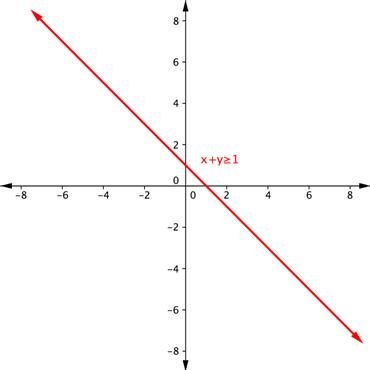
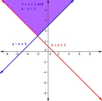
Shade the region of the graph that represents solutions for both inequalities. [latex]x+y\geq1[/latex] and [latex]y–x\geq5[/latex].


The videos that follow show more examples of graphing the solution set of a system of linear inequalities.
The system in our next example includes a compound inequality. We will see that you can treat a compound inequality like two lines when you are graphing them.
Example
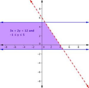
Find the solution to the system [latex]3x + 2y < 12[/latex] and [latex]-1 ≤ y ≤ 5[/latex].


In the video that follows, we show how to solve another system of inequalities that contains a compound inequality.
Try It
Systems with No Solutions
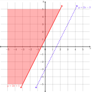
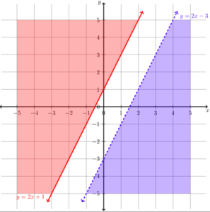
In the next example, we will show the solution to a system of two inequalities whose boundary lines are parallel to each other. When the graphs of a system of two linear equations are parallel to each other, we found that there was no solution to the system. We will get a similar result for the following system of linear inequalities.
Examples
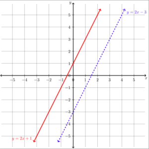
Graph the system [latex]\begin{array}{c}y\ge2x+1\\y\lt2x-3\end{array}[/latex]

Candela Citations
- Ex 1: Graph a System of Linear Inequalities. Authored by: James Sousa (Mathispower4u.com) . Located at: https://youtu.be/ACTxJv1h2_c. License: CC BY: Attribution
- Ex 2: Graph a System of Linear Inequalities. Authored by: James Sousa (Mathispower4u.com) . Located at: https://youtu.be/cclH2h1NurM. License: CC BY: Attribution
- Determine the Solution to a System of Inequalities (Compound). Authored by: James Sousa (Mathispower4u.com) . Located at: https://youtu.be/D-Cnt6m8l18. License: CC BY: Attribution
- Unit 14: Systems of Equations and Inequalities, from Developmental Math: An Open Program. Provided by: Monterey Institute of Technology. Located at: http://nrocnetwork.org/dm-opentext. License: CC BY: Attribution