Linear and Geometric Growth

Learning Outcomes

Determine whether data or a scenario describe linear or geometric growth
Identify growth rates, initial values, or point values expressed verbally, graphically, or numerically, and translate them into a format usable in calculation
Calculate recursive and explicit equations for linear and geometric growth given sufficient information, and use those equations to make predictions

Having a constant rate of change is the defining characteristic of linear growth. Plotting coordinate pairs associated with constant change will result in a straight line, the shape of linear growth. In this section, we will formalize a way to describe linear growth using mathematical terms and concepts. By the end of this section, you will be able to write both a recursive and explicit equations for linear growth given starting conditions, or a constant of change. You will also be able to recognize the difference between linear and geometric growth given a graph or an equation.

Linear (Algebraic) Growth

Predicting Growth

Marco is a collector of antique soda bottles. His collection currently contains 437 bottles. Every year, he budgets enough money to buy 32 new bottles. Can we determine how many bottles he will have in 5 years, and how long it will take for his collection to reach 1000 bottles?

While you could probably solve both of these questions without an equation or formal mathematics, we are going to formalize our approach to this problem to provide a means to answer more complicated questions.

Suppose that P_nrepresents the number, or population, of bottles Marco has after n years. So P₀ would represent the number of bottles now, P₁ would represent the number of bottles after 1 year, P₂ would represent the number of bottles after 2 years, and so on. We could describe how Marco’s bottle collection is changing using:

P₀ = 437

P_n = P_n-1 + 32

This is called a recursive relationship. A recursive relationship is a formula which relates the next value in a sequence to the previous values. Here, the number of bottles in year n can be found by adding 32 to the number of bottles in the previous year, P_n-1. Using this relationship, we could calculate:

P₁ = P₀ + 32 = 437 + 32 = 469

P₂ = P₁ + 32 = 469 + 32 = 501

P₃ = P₂ + 32 = 501 + 32 = 533

P₄ = P₃ + 32 = 533 + 32 = 565

P₅ = P₄ + 32 = 565 + 32 = 597

We have answered the question of how many bottles Marco will have in 5 years. 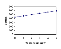Line chart. Vertical measures Bottles, with increments of 100 from 0 to 700. Horizontal measures Years From Now, with increments of 1 from 0 to 5. The line moves in a slow rise from left to right, from a little over 400 at year 0 to 600 at year 5.

However, solving how long it will take for his collection to reach 1000 bottles would require a lot more calculations.

While recursive relationships are excellent for describing simply and cleanly how a quantity is changing, they are not convenient for making predictions or solving problems that stretch far into the future. For that, a closed or explicit form for the relationship is preferred. An explicit equation allows us to calculate P_ndirectly, without needing to know P_n-1. While you may already be able to guess the explicit equation, let us derive it from the recursive formula. We can do so by selectively not simplifying as we go:

P₁ = 437 + 32 = 437 + 1(32)

P₂ = P₁ + 32 = 437 + 32 + 32 = 437 + 2(32)

P₃ = P₂ + 32 = (437 + 2(32)) + 32 = 437 + 3(32)

P₄ = P₃ + 32 = (437 + 3(32)) + 32 = 437 + 4(32)

You can probably see the pattern now, and generalize that

P_n = 437 + n(32) = 437 + 32n

Using this equation, we can calculate how many bottles he’ll have after 5 years:

P₅ = 437 + 32(5) = 437 + 160 = 597

We can now also solve for when the collection will reach 1000 bottles by substituting in 1000 for P_n and solving for n

1000 = 437 + 32_n

563 = 32_n

n = 563/32 = 17.59

So Marco will reach 1000 bottles in 18 years.

The steps of determining the formula and solving the problem of Marco’s bottle collection are explained in detail in the following videos.

In this example, Marco’s collection grew by the same number of bottles every year. This constant change is the defining characteristic of linear growth. Plotting the values we calculated for Marco’s collection, we can see the values form a straight line, the shape of linear growth.

Linear Growth

If a quantity starts at size P₀ and grows by d every time period, then the quantity after n time periods can be determined using either of these relations:

Recursive form

P_n = P_n-1 + d

Explicit form

P_n = P₀+ d n

In this equation, d represents the common difference – the amount that the population changes each time n increases by 1.

Connection to Prior Learning: Slope and Intercept

You may recognize the common difference, d, in our linear equation as slope. In fact, the entire explicit equation should look familiar – it is the same linear equation you learned in algebra, probably stated as y = mx + b.

In the standard algebraic equation y = mx + b, b was the y-intercept, or the y value when x was zero. In the form of the equation we’re using, we are using P0 to represent that initial amount.

In the y = mx + b equation, recall that m was the slope. You might remember this as “rise over run,” or the change in y divided by the change in x. Either way, it represents the same thing as the common difference, d, we are using – the amount the output P_n changes when the input n increases by 1.

The equations y = mx + b and P_n = P₀+ d n mean the same thing and can be used the same ways. We’re just writing it somewhat differently.

Examples

The population of elk in a national forest was measured to be 12,000 in 2003, and was measured again to be 15,000 in 2007. If the population continues to grow linearly at this rate, what will the elk population be in 2014?

Show Solution

View more about this example here.

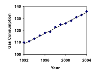
Gasoline consumption in the US has been increasing steadily. Consumption data from 1992 to 2004 is shown below.^[1] Find a model for this data, and use it to predict consumption in 2016. If the trend continues, when will consumption reach 200 billion gallons?

Year	’92	’93	’94	’95	’96	’97	’98	’99	’00	’01	’02	’03	’04
Consumption (billion of gallons)	110	111	113	116	118	119	123	125	126	128	131	133	136

Show Solution

Plotting this data, it appears to have an approximately linear relationship:

Graph. Vertical measures Gas Consumption in increments of 10, from 100 to 140. Horizontal measures Year in increments of 4, from 1992 to 2004. Points identified in a generally upward trend, left to right, from 110 in 1992 to near 140 in 2004.

While there are more advanced statistical techniques that can be used to find an equation to model the data, to get an idea of what is happening, we can find an equation by using two pieces of the data – perhaps the data from 1993 and 2003.

Letting n = 0 correspond with 1993 would give P₀ = 111 billion gallons.

To find d, we need to know how much the gas consumption increased each year, on average. From 1993 to 2003 the gas consumption increased from 111 billion gallons to 133 billion gallons, a total change of 133 – 111 = 22 billion gallons, over 10 years. This gives us an average change of 22 billion gallons / 10 year = 2.2 billion gallons per year.

Equivalently,

[latex]d=slope=\frac{\text{changeinoutput}}{\text{changeininput}}=\frac{133-111}{10-0}=\frac{22}{10}=2.2[/latex]billion gallons per year

We can now write our equation in whichever form is preferred.

Recursive form

P₀ = 111

P_n = P_n-1 + 2.2

Explicit form

P_n = 111 + 2.2_n

Calculating values using the explicit form and plotting them with the original data shows how well our model fits the data.

We can now use our model to make predictions about the future, assuming that the previous trend continues unchanged. To predict the gasoline consumption in 2016:

n = 23 (2016 – 1993 = 23 years later)

P₂₃ = 111 + 2.2(23) = 161.6

Our model predicts that the US will consume 161.6 billion gallons of gasoline in 2016 if the current trend continues.

To find when the consumption will reach 200 billion gallons, we would set P_n= 200, and solve for n:

P_n = 200 Replace P_n with our model

111 + 2.2_n = 200 Subtract 111 from both sides

2.2_n = 89 Divide both sides by 2.2

n = 40.4545

This tells us that consumption will reach 200 billion about 40 years after 1993, which would be in the year 2033.

The steps for reaching this answer are detailed in the following video.

The cost, in dollars, of a gym membership for n months can be described by the explicit equation P_n = 70 + 30_n. What does this equation tell us?

Show Solution

The explanation for this example is detailed below.

Try It

The number of stay-at-home fathers in Canada has been growing steadily^[2]. While the trend is not perfectly linear, it is fairly linear. Use the data from 1976 and 2010 to find an explicit formula for the number of stay-at-home fathers, then use it to predict the number in 2020.

Year	1976	1984	1991	2000	2010
# of Stay -at-home fathers	20610	28725	43530	47665	53555

Show Solution

When Good Models Go Bad

When using mathematical models to predict future behavior, it is important to keep in mind that very few trends will continue indefinitely.

Example

Suppose a four year old boy is currently 39 inches tall, and you are told to expect him to grow 2.5 inches a year.

We can set up a growth model, with n = 0 corresponding to 4 years old.

Recursive form

P₀ = 39

P_n = P_n-1 + 2.5

Explicit form

P_n = 39 + 2.5(n)

So at 6 years old, we would expect him to be

P₂ = 39 + 2.5(2) = 44 inches tall

Any mathematical model will break down eventually. Certainly, we shouldn’t expect this boy to continue to grow at the same rate all his life. If he did, at age 50 he would be

P₄₆ = 39 + 2.5(46) = 154 inches tall = 12.8 feet tall!

When using any mathematical model, we have to consider which inputs are reasonable to use. Whenever we extrapolate, or make predictions into the future, we are assuming the model will continue to be valid.

View a video explanation of this breakdown of the linear growth model here.

Exponential (Geometric ) Growth

Population Growth

Suppose that every year, only 10% of the fish in a lake have surviving offspring. If there were 100 fish in the lake last year, there would now be 110 fish. If there were 1000 fish in the lake last year, there would now be 1100 fish. Absent any inhibiting factors, populations of people and animals tend to grow by a percent of the existing population each year.

Suppose our lake began with 1000 fish, and 10% of the fish have surviving offspring each year. Since we start with 1000 fish, P₀ = 1000. How do we calculate P₁? The new population will be the old population, plus an additional 10%. Symbolically:

P₁ = P₀ + 0.10P₀

Notice this could be condensed to a shorter form by factoring:

P₁ = P₀ + 0.10P₀ = 1P₀ + 0.10P₀= (1+ 0.10)P₀= 1.10P₀

While 10% is the growth rate, 1.10 is the growth multiplier. Notice that 1.10 can be thought of as “the original 100% plus an additional 10%.”

For our fish population,

P₁ = 1.10(1000) = 1100

We could then calculate the population in later years:

P₂ = 1.10P₁ = 1.10(1100) = 1210

P₃ = 1.10P₂ = 1.10(1210) = 1331

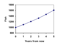
Notice that in the first year, the population grew by 100 fish; in the second year, the population grew by 110 fish; and in the third year the population grew by 121 fish.

While there is a constant percentage growth, the actual increase in number of fish is increasing each year.

Graphing these values we see that this growth doesn’t quite appear linear.

Line graph. Measured vertically: Fish, in increments of 200, from 800 to 1800. Measured horizontally: Years from now, measured in units of 1, from 0 to 5. Year 0 is at 1000; Year 1 is at roughly 1100; and subsequent years move in an increasing rate so that the overall line is curved to the upper right.

A walkthrough of this fish scenario can be viewed here:

To get a better picture of how this percentage-based growth affects things, we need an explicit form, so we can quickly calculate values further out in the future.

Like we did for the linear model, we will start building from the recursive equation:

P₁ = 1.10(P₀ )= 1.10(1000)

P₂ = 1.10(P₁ )= 1.10(1.10(1000)) = 1.102(1000)

P₃ = 1.10(P₂ )= 1.10(1.10²(1000)) = 1.103(1000)

P₄ = 1.10(P₃ )= 1.10(1.10³(1000)) = 1.104(1000)

Observing a pattern, we can generalize the explicit form to be:

P_n = 1.10ⁿ(1000), or equivalently, P_n = 1000(1.10ⁿ)

From this, we can quickly calculate the number of fish in 10, 20, or 30 years:

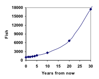
Line graph. Measured vertically: Fish, in increments of 3000, from 0 to 18,000. Measured horizontally: Years from now, measured in units of 5, from 0 to 30. Year 0 is at 1000, with a tight cluster of dots in the lower left quadrant. The exponential increase becomes more dramatic as time advances, so that year 30 is at 18,000 fish with more spacing between dots.

P₁₀ = 1.10¹⁰(1000) = 2594

P₂₀ = 1.10²⁰(1000) = 6727

P₃₀ = 1.10³⁰(1000) = 17449

Adding these values to our graph reveals a shape that is definitely not linear. If our fish population had been growing linearly, by 100 fish each year, the population would have only reached 4000 in 30 years, compared to almost 18,000 with this percent-based growth, called exponential growth.

A video demonstrating the explicit model of this fish story can be viewed here:

In exponential growth, the population grows proportional to the size of the population, so as the population gets larger, the same percent growth will yield a larger numeric growth.

Exponential Growth

If a quantity starts at size P₀ and grows by R% (written as a decimal, r) every time period, then the quantity after n time periods can be determined using either of these relations:

Recursive form

P_n = (1+r) P_n-1

Explicit form

P_n = (1+r)ⁿ P₀ or equivalently, P_n = P₀ (1+r)ⁿ

We call r the growth rate.

The term (1+r) is called the growth multiplier, or common ratio.

Example

Between 2007 and 2008, Olympia, WA grew almost 3% to a population of 245 thousand people. If this growth rate was to continue, what would the population of Olympia be in 2014?

Show Solution

The following video explains this example in detail.

Evaluating exponents on the calculator

To evaluate expressions like (1.03)⁶, it will be easier to use a calculator than multiply 1.03 by itself six times. Most scientific calculators have a button for exponents. It is typically either labeled like:

^ , y^x , or x^y .

To evaluate 1.03⁶ we’d type 1.03 ^ 6, or 1.03 y^x 6. Try it out – you should get an answer around 1.1940523.

Try It

India is the second most populous country in the world, with a population in 2008 of about 1.14 billion people. The population is growing by about 1.34% each year. If this trend continues, what will India’s population grow to by 2020?

Show Solution

Examples

A friend is using the equation P_n = 4600(1.072)ⁿto predict the annual tuition at a local college. She says the formula is based on years after 2010. What does this equation tell us?

Show Solution

View the following to see this example worked out.

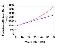
In 1990, residential energy use in the US was responsible for 962 million metric tons of carbon dioxide emissions. By the year 2000, that number had risen to 1182 million metric tons^[3]. If the emissions grow exponentially and continue at the same rate, what will the emissions grow to by 2050?

Show Solution

View more about this example here.

Rounding

As a note on rounding, notice that if we had rounded the growth rate to 2.1%, our calculation for the emissions in 2050 would have been 3347. Rounding to 2% would have changed our result to 3156. A very small difference in the growth rates gets magnified greatly in exponential growth. For this reason, it is recommended to round the growth rate as little as possible.

If you need to round, keep at least three significant digits – numbers after any leading zeros. So 0.4162 could be reasonably rounded to 0.416. A growth rate of 0.001027 could be reasonably rounded to 0.00103.

Evaluating roots on the calculator

In the previous example, we had to calculate the 10th root of a number. This is different than taking the basic square root, √. Many scientific calculators have a button for general roots. It is typically labeled like:

[latex]\sqrt[y]{x}[/latex]

To evaluate the 3rd root of 8, for example, we’d either type 3 [latex]\sqrt[x]{{}}[/latex] 8, or 8 [latex]\sqrt[x]{{}}[/latex] 3, depending on the calculator. Try it on yours to see which to use – you should get an answer of 2.

If your calculator does not have a general root button, all is not lost. You can instead use the property of exponents which states that:

[latex]\sqrt[n]{a}={a}^{\frac{1}{2}}[/latex].

So, to compute the 3rd root of 8, you could use your calculator’s exponent key to evaluate 8^1/3. To do this, type:

8 y^x ( 1 ÷ 3 )

The parentheses tell the calculator to divide 1/3 before doing the exponent.

Try It

The number of users on a social networking site was 45 thousand in February when they officially went public, and grew to 60 thousand by October. If the site is growing exponentially, and growth continues at the same rate, how many users should they expect two years after they went public?

Show Solution

Example

Looking back at the last example, for the sake of comparison, what would the carbon emissions be in 2050 if emissions grow linearly at the same rate?

Show Solution

A demonstration of this example can be seen in the following video.

So how do we know which growth model to use when working with data? There are two approaches which should be used together whenever possible:

Find more than two pieces of data. Plot the values, and look for a trend. Does the data appear to be changing like a line, or do the values appear to be curving upwards?
Consider the factors contributing to the data. Are they things you would expect to change linearly or exponentially? For example, in the case of carbon emissions, we could expect that, absent other factors, they would be tied closely to population values, which tend to change exponentially.

Module 8: Growth Models

Learning Outcomes

Linear (Algebraic) Growth

Predicting Growth

Linear Growth

Recursive form

Explicit form

Connection to Prior Learning: Slope and Intercept

Examples

Recursive form

Explicit form

Recursive form

Explicit form

Try It

When Good Models Go Bad

Example

Recursive form

Explicit form

Exponential (Geometric ) Growth

Population Growth

Exponential Growth

Recursive form

Explicit form

Example

Evaluating exponents on the calculator

Try It

Examples

Rounding

Evaluating roots on the calculator

Try It

Example