Natural Logarithms

Learning Outcomes

Write the definition of the natural logarithm as an integral
Recognize the derivative of the natural logarithm
Integrate functions involving the natural logarithmic function
Define the number 𝑒 through an integral

The Natural Logarithm as an Integral

Recall the power rule for integrals:

\int x^{n} d x = \frac{x^{n + 1}}{n + 1} + C, n \neq - 1.

$\displaystyle\int {x}^{n}dx=\frac{{x}^{n+1}}{n+1}+C,n\ne \text{−}1.$

Clearly, this does not work when $n=-1,$ as it would force us to divide by zero. So, what do we do with $\displaystyle\int \frac{1}{x}dx?$ Recall from the Fundamental Theorem of Calculus that ${\displaystyle\int }_{1}^{x}\dfrac{1}{t}dt$ is an antiderivative of $\frac{1}{x}.$ Therefore, we can make the following definition.

Definition

For $x>0,$ define the natural logarithm function by

ln x = \int_{1}^{x} \frac{1}{t} d t

$\text{ln}x={\displaystyle\int }_{1}^{x}\frac{1}{t}dt$

For $x>1,$ this is just the area under the curve $y=1\text{/}t$ from 1 to $x.$ For $x<1,$ we have ${\displaystyle\int }_{1}^{x}\frac{1}{t}dt=\text{−}{\displaystyle\int }_{x}^{1}\frac{1}{t}dt,$ so in this case it is the negative of the area under the curve from $x\text{ to }1$ (see the following figure).

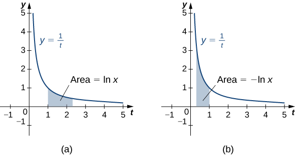
This figure has two graphs. The first is the curve y=1/t. It is decreasing and in the first quadrant. Under the curve is a shaded area. The area is bounded to the left at x=1. The area is labeled “area=lnx”. The second graph is the same curve y=1/t. It has shaded area under the curve bounded to the right by x=1. It is labeled “area=-lnx”.

Figure 1. (a) When $x>1,$ the natural logarithm is the area under the curve $y=\frac{1}{t}$ from $1\text{ to }x.$ (b) When $x<1,$ the natural logarithm is the negative of the area under the curve from $x$ to 1.

Notice that $\text{ln}1=0.$ Furthermore, the function $y=\frac{1}{t}>0$ for $x>0.$ Therefore, by the properties of integrals, it is clear that $\text{ln}x$ is increasing for $x>0.$

Properties of the Natural Logarithm

Because of the way we defined the natural logarithm, the following differentiation formula falls out immediately as a result of to the Fundamental Theorem of Calculus.

Derivative of the Natural Logarithm

For $x>0,$ the derivative of the natural logarithm is given by

\frac{d}{d x} ln x = \frac{1}{x} .

$\frac{d}{dx}\text{ln}x=\dfrac{1}{x}.$

Corollary to the Derivative of the Natural Logarithm

The function $\text{ln}x$ is differentiable; therefore, it is continuous.

A graph of $\text{ln}x$ is shown in Figure 2. Notice that it is continuous throughout its domain of $(0,\infty ).$

This figure is a graph. It is an increasing curve labeled f(x)=lnx. The curve is increasing with the y-axis as an asymptote. The curve intersects the x-axis at x=1.

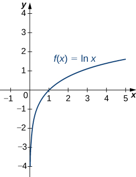
Figure 2. The graph of $f(x)=\text{ln}x$ shows that it is a continuous function.

Example: Calculating Derivatives of Natural Logarithms

Calculate the following derivatives:

$\frac{d}{dx}\text{ln}(5{x}^{3}-2)$
$\frac{d}{dx}{(\text{ln}(3x))}^{2}$

Show Solution

We need to apply the chain rule in both cases.

$\frac{d}{dx}\text{ln}(5{x}^{3}-2)=\frac{15{x}^{2}}{5{x}^{3}-2}$
$\frac{d}{dx}{(\text{ln}(3x))}^{2}=\frac{2(\text{ln}(3x))·3}{3x}=\frac{2(\text{ln}(3x))}{x}$

Try It

Calculate the following derivatives:

$\frac{d}{dx}\text{ln}(2{x}^{2}+x)$
$\frac{d}{dx}{(\text{ln}({x}^{3}))}^{2}$

Hint

Show Solution

$\frac{d}{dx}\text{ln}(2{x}^{2}+x)=\frac{4x+1}{2{x}^{2}+x}$
$\frac{d}{dx}{(\text{ln}({x}^{3}))}^{2}=\frac{6\text{ln}({x}^{3})}{x}$

Watch the following video to see the worked solution to the above Try It.

Closed Captioning and Transcript Information for Video

Try It

Note that if we use the absolute value function and create a new function $\text{ln}|x|,$ we can extend the domain of the natural logarithm to include $x<0.$ Then $(d\text{/}(dx))\text{ln}|x|=1\text{/}x.$ This gives rise to the familiar integration formula.

Integral of (1/ $u$ ) du

The natural logarithm is the antiderivative of the function $f(u)=1\text{/}u\text{:}$

\int \frac{1}{u} d u = ln | u | + C

$\displaystyle\int \frac{1}{u}du=\text{ln}|u|+C$

Example: Calculating Integrals Involving Natural Logarithms

Calculate the integral $\displaystyle\int \frac{x}{{x}^{2}+4}dx.$

Show Solution

Using $u$ -substitution, let $u={x}^{2}+4.$ Then $du=2xdx$ and we have

\int \frac{x}{x^{2} + 4} d x = \frac{1}{2} \int \frac{1}{u} d u \frac{1}{2} ln | u | + C = \frac{1}{2} ln | x^{2} + 4 | + C = \frac{1}{2} ln (x^{2} + 4) + C .

$\displaystyle\int \frac{x}{{x}^{2}+4}dx=\frac{1}{2}\displaystyle\int \frac{1}{u}du\frac{1}{2}\text{ln}|u|+C=\frac{1}{2}\text{ln}|{x}^{2}+4|+C=\frac{1}{2}\text{ln}({x}^{2}+4)+C.$

Try It

Calculate the integral $\displaystyle\int \frac{{x}^{2}}{{x}^{3}+6}dx.$

Hint

Apply the integration formula provided earlier and use

u

$u$ -substitution as necessary.

Show Solution

$\displaystyle\int \frac{{x}^{2}}{{x}^{3}+6}dx=\frac{1}{3}\text{ln}|{x}^{3}+6|+C$

Watch the following video to see the worked solution to the above Try It.

Closed Captioning and Transcript Information for Video

Try It

Although we have called our function a “logarithm,” we have not actually proved that any of the properties of logarithms hold for this function. We do so here.

Properties of the Natural Logarithm

If $a,b>0$ and $r$ is a rational number, then

$\text{ln}1=0$
$\text{ln}(ab)=\text{ln}a+\text{ln}b$
$\text{ln}(\frac{a}{b})=\text{ln}a-\text{ln}b$
$\text{ln}({a}^{r})=r\text{ln}a$

Proof

By definition, $\text{ln}1={\displaystyle\int }_{1}^{1}\frac{1}{t}dt=0.$
We have
$\text{ln}(ab)={\displaystyle\int }_{1}^{ab}\frac{1}{t}dt={\displaystyle\int }_{1}^{a}\frac{1}{t}dt+{\displaystyle\int }_{a}^{ab}\frac{1}{t}dt.$

Use $u\text{-substitution}$ on the last integral in this expression. Let $u=t\text{/}a.$ Then $du=(1\text{/}a)dt.$ Furthermore, when $t=a,u=1,$ and when $t=ab,u=b.$ So we get

$\text{ln}(ab)={\displaystyle\int }_{1}^{a}\frac{1}{t}dt+{\displaystyle\int }_{a}^{ab}\frac{1}{t}dt={\displaystyle\int }_{1}^{a}\frac{1}{t}dt+{\displaystyle\int }_{1}^{ab}\frac{a}{t}·\frac{1}{a}dt={\displaystyle\int }_{1}^{a}\frac{1}{t}dt+{\displaystyle\int }_{1}^{b}\frac{1}{u}du=\text{ln}a+\text{ln}b.$
Note that
$\frac{d}{dx}\text{ln}({x}^{r})=\frac{r{x}^{r-1}}{{x}^{r}}=\frac{r}{x}.$

Furthermore,

$\frac{d}{dx}(r\text{ln}x)=\frac{r}{x}.$

Since the derivatives of these two functions are the same, by the Fundamental Theorem of Calculus, they must differ by a constant. So we have

$\text{ln}({x}^{r})=r\text{ln}x+C$

for some constant $C.$ Taking $x=1,$ we get

$\begin{array}{ccc}\hfill \text{ln}({1}^{r})& =\hfill & r\text{ln}(1)+C\hfill \\ \hfill 0& =\hfill & r(0)+C\hfill \\ \hfill C& =\hfill & 0.\hfill \end{array}$

Thus $\text{ln}({x}^{r})=r\text{ln}x$ and the proof is complete. Note that we can extend this property to irrational values of $r$ later in this section.
Part iii. follows from parts ii. and iv. and the proof is left to you.

$_\blacksquare$

Example: Using Properties of Logarithms

Use properties of logarithms to simplify the following expression into a single logarithm:

$\text{ln}9-2\text{ln}3+\text{ln}(\frac{1}{3})$

Show Solution

We have

$\text{ln}9-2\text{ln}3+\text{ln}(\frac{1}{3})=\text{ln}({3}^{2})-2\text{ln}3+\text{ln}({3}^{-1})=2\text{ln}3-2\text{ln}3-\text{ln}3=\text{−}\text{ln}3.$

Try It

Use properties of logarithms to simplify the following expression into a single logarithm:

$\text{ln}8-\text{ln}2-\text{ln}(\frac{1}{4}).$

Hint

Show Solution

$4\text{ln}2$

Defining the Number $e$

Now that we have the natural logarithm defined, we can use that function to define the number $e.$

Definition

The number $e$ is defined to be the real number such that

$\text{ln}e=1$

To put it another way, the area under the curve $y=1\text{/}t$ between $t=1$ and $t=e$ is 1 (Figure 3). The proof that such a number exists and is unique is left to you. (Hint: Use the Intermediate Value Theorem to prove existence and the fact that $\text{ln}x$ is increasing to prove uniqueness.)

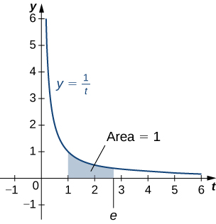
This figure is a graph. It is the curve y=1/t. It is decreasing and in the first quadrant. Under the curve is a shaded area. The area is bounded to the left at x=1 and to the right at x=e. The area is labeled “area=1”.

Figure 3. The area under the curve from 1 to $e$ is equal to one.

The number $e$ can be shown to be irrational, although we won’t do so here (see the activity in Taylor and Maclaurin Series in Calculus 2). Its approximate value is given by

$e\approx 2.71828182846$

Module 2: Applications of Integration

Learning Outcomes

The Natural Logarithm as an Integral

Definition

Properties of the Natural Logarithm

Derivative of the Natural Logarithm

Corollary to the Derivative of the Natural Logarithm

Example: Calculating Derivatives of Natural Logarithms

Try It

Try It

Integral of (1/ $u$ ) du

Example: Calculating Integrals Involving Natural Logarithms

Try It

Try It

Properties of the Natural Logarithm

Proof

Example: Using Properties of Logarithms

Try It

Defining the Number $e$

Definition

Candela Citations

Module 2: Applications of Integration