Learning Outcomes
- Use Riemann sums to approximate area
So far we have been using rectangles to approximate the area under a curve. The heights of these rectangles have been determined by evaluating the function at either the right or left endpoints of the subinterval [latex][x_{i-1},x_i][/latex]. In reality, there is no reason to restrict evaluation of the function to one of these two points only. We could evaluate the function at any point [latex]x_i^*[/latex] in the subinterval [latex][x_{i-1},x_i][/latex], and use [latex]f(x_i^*)[/latex] as the height of our rectangle. This gives us an estimate for the area of the form
A sum of this form is called a Riemann sum, named for the 19th-century mathematician Bernhard Riemann, who developed the idea.
Definition
Let [latex]f(x)[/latex] be defined on a closed interval [latex][a,b][/latex] and let [latex]P[/latex] be a regular partition of [latex][a,b][/latex]. Let [latex]\Delta x[/latex] be the width of each subinterval [latex][x_{i-1},x_i][/latex] and for each [latex]i[/latex], let [latex]x_i^*[/latex] be any point in [latex][x_{i-1},x_i][/latex]. A Riemann sum is defined for [latex]f(x)[/latex] as
Recall that with the left- and right-endpoint approximations, the estimates seem to get better and better as [latex]n[/latex] get larger and larger. The same thing happens with Riemann sums. Riemann sums give better approximations for larger values of [latex]n[/latex]. We are now ready to define the area under a curve in terms of Riemann sums.
Definition
Let [latex]f(x)[/latex] be a continuous, nonnegative function on an interval [latex][a,b][/latex], and let [latex]\displaystyle\sum_{i=1}^{n} f(x_i^*)\Delta x[/latex] be a Riemann sum for [latex]f(x)[/latex]. Then, the area under the curve [latex]y=f(x)[/latex] on [latex][a,b][/latex] is given by
Some subtleties here are worth discussing. First, note that taking the limit of a sum is a little different from taking the limit of a function [latex]f(x)[/latex] as [latex]x[/latex] goes to infinity. Limits of sums are discussed in detail in the chapter on Sequences and Series in the second volume of this text; however, for now we can assume that the computational techniques we used to compute limits of functions can also be used to calculate limits of sums.
Second, we must consider what to do if the expression converges to different limits for different choices of [latex]\{x_i^*\}[/latex]. Fortunately, this does not happen. Although the proof is beyond the scope of this text, it can be shown that if [latex]f(x)[/latex] is continuous on the closed interval [latex][a,b][/latex], then [latex]\underset{n\to \infty }{\lim}\displaystyle\sum_{i=1}^{n} f(x_i^*)\Delta x[/latex] exists and is unique (in other words, it does not depend on the choice of [latex]\{x_i^*\}[/latex]).
We look at some examples shortly. But, before we do, let’s take a moment and talk about some specific choices for [latex]\{x_i^*\}[/latex]. Although any choice for [latex]\{x_i^*\}[/latex] gives us an estimate of the area under the curve, we don’t necessarily know whether that estimate is too high (overestimate) or too low (underestimate). If it is important to know whether our estimate is high or low, we can select our value for [latex]\{x_i^*\}[/latex] to guarantee one result or the other.
If we want an overestimate, for example, we can choose [latex]\{x_i^*\}[/latex] such that for [latex]i=1,2,3,\cdots,n, \, f(x_i^*)\ge f(x)[/latex] for all [latex]x\in [x_{i-1},x_i][/latex]. In other words, we choose [latex]\{x_i^*\}[/latex] so that for [latex]i=1,2,3,\cdots,n, \, f(x_i^*)[/latex] is the maximum function value on the interval [latex][x_{i-1},x_i][/latex]. If we select [latex]\{x_i^*\}[/latex] in this way, then the Riemann sum [latex]\displaystyle\sum_{i=1}^{n} f(x_i^*)\Delta x[/latex] is called an upper sum. Similarly, if we want an underestimate, we can choose [latex]\{x_i^*\}[/latex] so that for [latex]i=1,2,3,\cdots,n, \, f(x_i^*)[/latex] is the minimum function value on the interval [latex][x_{i-1},x_i][/latex]. In this case, the associated Riemann sum is called a lower sum. Note that if [latex]f(x)[/latex] is either increasing or decreasing throughout the interval [latex][a,b][/latex], then the maximum and minimum values of the function occur at the endpoints of the subintervals, so the upper and lower sums are just the same as the left- and right-endpoint approximations.
Tip: If a function is increasing over a closed interval, the right endpoints will be used to calculate the upper sum and the left endpoints the lower sum. If a function is decreasing over a closed interval, the right endpoints will be used for the lower sum and the left endpoints the upper sum.
example: Finding Lower and Upper Sums
Find a lower sum for [latex]f(x)=10-x^2[/latex] on [latex][1,2][/latex]; use [latex]n=4[/latex] subintervals.
![The graph of f(x) = 10 − x^2 from 0 to 2. It is set up for a right-end approximation of the area bounded by the curve and the x-axis on [1, 2], labeled a=x0 to x4. It shows a lower sum.](https://s3-us-west-2.amazonaws.com/courses-images/wp-content/uploads/sites/2332/2018/01/11203921/CNX_Calc_Figure_05_01_014.jpg)
Watch the following video to see the worked solution to Example: Finding Lower and Upper Sums.
Try It
- Find an upper sum for [latex]f(x)=10-x^2[/latex] on [latex][1,2][/latex]; let [latex]n=4[/latex].
- Sketch the approximation.
![A graph of the function f(x) = 10 − x^2 from 0 to 2. It is set up for a right endpoint approximation over the area [1,2], which is labeled a=x0 to x4. It is an upper sum.](https://s3-us-west-2.amazonaws.com/courses-images/wp-content/uploads/sites/2332/2018/01/11203924/CNX_Calc_Figure_05_01_015.jpg)
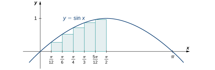
Example: Finding Lower and Upper Sums for [latex]f(x)= \sin x[/latex]
Find a lower sum for [latex]f(x)= \sin x[/latex] over the interval [latex][a,b]=[0,\frac{\pi }{2}][/latex]; let [latex]n=6[/latex].
Watch the following video to see the worked solution to Example: Finding Lower and Upper Sums for [latex]f(x)= \sin x[/latex].
Try It
Using the function [latex]f(x)= \sin x[/latex] over the interval [latex][0,\frac{\pi}{2}][/latex], find an upper sum; let [latex]n=6[/latex].
Try It
Candela Citations
- 5.1 Approximating Areas. Authored by: Ryan Melton. License: CC BY: Attribution
- Calculus Volume 2. Authored by: Gilbert Strang, Edwin (Jed) Herman. Provided by: OpenStax. Located at: https://openstax.org/books/calculus-volume-2/pages/1-introduction. License: CC BY-NC-SA: Attribution-NonCommercial-ShareAlike. License Terms: Access for free at https://openstax.org/books/calculus-volume-2/pages/1-introduction
